Coupled ocean-atmosphere model (MAOOAM)

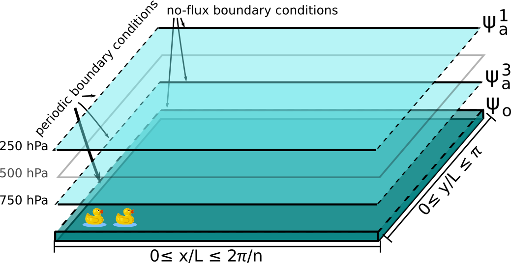
This model version is composed of a two-layer quasi-geostrophic Atmospheric component coupled both thermally and mechanically to a shallow-water Oceanic component. The coupling between the two components includes wind forcings, radiative and heat exchanges.

../../_images/model_variables_duck.png

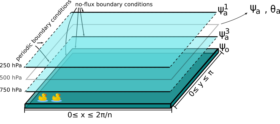
Sketch of the ocean-atmosphere coupled model layers. The atmosphere is here a periodic channel while the ocean is a closed basin. The domain (\(\beta\)-plane) zonal and meridional coordinates are labeled as the \(x\) and \(y\) variables.

The evolution equations for the atmospheric and oceanic streamfunctions defined in the sections above read

\[\begin{split}\frac{\partial}{\partial t} \left(\nabla^2 \psi^1_{\rm a}\right)+ J(\psi^1_{\rm a}, \nabla^2 \psi^1_{\rm a})+ \beta \frac{\partial \psi^1_{\rm a}}{\partial x} & = -k'_d \nabla^2 (\psi^1_{\rm a}-\psi^3_{\rm a})+ \frac{f_0}{\Delta p} \omega \nonumber \\ \frac{\partial}{\partial t} \left( \nabla^2 \psi^3_{\rm a} \right) + J(\psi^3_{\rm a}, \nabla^2 \psi^3_{\rm a}) + \beta \frac{\partial \psi^3_{\rm a}}{\partial x} & = +k'_d \nabla^2 (\psi^1_{\rm a}-\psi^3_{\rm a}) - \frac{f_0}{\Delta p} \omega \nonumber - k_d \nabla^2 \left(\psi^3_{\rm a} - \psi_{\rm o}\right) \\ \frac{\partial}{\partial t} \left( \nabla^2 \psi_\text{o} - \frac{\psi_\text{o}}{L_\text{R}^2} \right) + J(\psi_\text{o}, \nabla^2 \psi_\text{o}) + \beta \frac{\partial \psi_\text{o}}{\partial x} & = -r \nabla^2 \psi_\text{o} +\frac{C}{\rho_{\rm o} h} \nabla^2 (\psi^3_\text{a}-\psi_\text{o}).\nonumber\end{split}\]

where \(\rho_{\rm o}\) is the density of the ocean’s water and \(h\) is the depth of its layer (h). The rightmost term of the last equation represents the impact of the wind stress on the ocean, and is modulated by the coefficient of the mechanical ocean-atmosphere coupling, \(d = C/(\rho_{\rm o} h)\) (d).

As we did for the Model with an orography and a temperature profile, we rewrite these equations in terms of the barotropic streamfunction \(\psi_{\rm a}\) and baroclinic streamfunction \(\theta_{\rm a}\):

\[\begin{split}&\frac{\partial}{\partial t} \left(\nabla^2 \psi_{\rm a}\right) + J(\psi_{\rm a}, \nabla^2 \psi_{\rm a}) + J(\theta_{\rm a}, \nabla^2 \theta_{\rm a}) + \beta \frac{\partial \psi_{\rm a}}{\partial x} = - \frac{k_d}{2} \nabla^2 (\psi_{\rm a} - \theta_{\rm a} - \psi_{\rm o}) \\ &\frac{\partial}{\partial t} \left( \nabla^2 \theta_{\rm a} \right) + J(\psi_{\rm a}, \nabla^2 \theta_{\rm a}) + J(\theta_{\rm a}, \nabla^2 \psi_{\rm a}) + \beta \frac{\partial \theta_{\rm a}}{\partial x} \nonumber \\ & \qquad \qquad \qquad \qquad \qquad \qquad = - 2 \, k'_d \nabla^2 \theta_{\rm a} + \frac{k_d}{2} \nabla^2 (\psi_{\rm a} - \theta_{\rm a} - \psi_{\rm o}) + \frac{f_0}{\Delta p} \omega \nonumber \\ &\frac{\partial}{\partial t} \left( \nabla^2 \psi_\text{o} - \frac{\psi_\text{o}}{L_\text{R}^2} \right) + J(\psi_\text{o}, \nabla^2 \psi_\text{o}) + \beta \frac{\partial \psi_\text{o}}{\partial x} = -r \nabla^2 \psi_\text{o} + d \, \nabla^2 (\psi_\text{a}- \theta_\text{a}-\psi_\text{o}).\nonumber\end{split}\]

Temperature equations

The temperature \(T_\text{o}\) in the ocean is a passively advected scalar interacting with the atmospheric temperature through radiative and heat exchange, according to a scheme detailed in [BB98]:

\[\gamma_\text{o} \left( \frac{\partial T_\text{o}}{\partial t} + J(\psi_\text{o}, T_\text{o}) \right) = -\lambda (T_\text{o}-T_\text{a}) -\sigma_\text{B} T_\text{o}^4 + \epsilon_\text{a} \sigma_\text{B} T_\text{a}^4 + R_\text{o}\]

and the time evolution of the atmospheric temperature \(T_\text{a}\) obeys a similar equation:

\[\gamma_\text{a} \left( \frac{\partial T_\text{a}}{\partial t} + J(\psi_\text{a}, T_\text{a}) -\sigma \omega \frac{p}{R}\right) = -\lambda (T_\text{a}-T_\text{o}) + \epsilon_\text{a} \sigma_\text{B} T_\text{o}^4 - 2 \epsilon_\text{a} \sigma_\text{B} T_\text{a}^4 + R_\text{a}\]

where \(\gamma_\text{a}\) (AtmosphericTemperatureParams.gamma) and \(\gamma_\text{o}\) (OceanicTemperatureParams.gamma) are the heat capacities of the atmosphere and the active ocean layer. \(\lambda\) (hlambda) is the heat transfer coefficient at the ocean-atmosphere interface. \(\sigma\) (sigma) is the static stability of the atmosphere, taken to be constant. The quartic terms represent the long-wave radiation fluxes between the ocean, the atmosphere, and outer space, with \(\epsilon_\text{a}\) (eps) the emissivity of the grey-body atmosphere and \(\sigma_\text{B}\) (sb) the Stefan–Boltzmann constant. By decomposing the temperatures as \(T_\text{a} = T_{\text{a},0} + \delta T_\text{a}\) and \(T_\text{o} = T_{\text{o},0} + \delta T_\text{o}\), the quartic terms are linearized around spatially uniform and constant temperatures \(T_{\text{a},0}\) (AtmosphericTemperatureParams.T0) and \(T_{\text{o},0}\) (OceanicTemperatureParams.T0), as detailed in Appendix B of [VDDCG15]. \(R_\text{a}\) and \(R_\text{o}\) are the short-wave radiation fluxes entering the atmosphere and the ocean that are also decomposed as \(R_\text{a}=R_{\text{a}, 0} + \delta R_\text{a}\) and \(R_\text{o} = R_{\text{o}, 0} + \delta R_\text{o}\). It results in these evolution equations for the temperature anomalies:

\[\begin{split}\gamma_{\rm a} \Big( \frac{\partial \delta T_{\rm a}}{\partial t} + J(\psi_{\rm a}, \delta T_{\rm a} )- \sigma \omega \frac{p}{R}\Big) &= -\lambda (\delta T_{\rm a}- \delta T_{\rm o}) +4 \sigma_B T_{{\rm o},0}^3 \delta T_{\rm o} - 8 \epsilon_{\rm a} \sigma_B T_{{\rm a},0}^3 \delta T_{\rm a} + \delta R_{\rm a} \nonumber \\ \gamma_{\rm o} \Big( \frac{\partial \delta T_{\rm o}}{\partial t} + J(\psi_{\rm o}, \delta T_{\rm o})\Big) &= -\lambda (\delta T_{\rm o}- \delta T_{\rm a}) -4 \sigma_B T_{{\rm o},0}^3 \delta T_{\rm o} + 4 \epsilon_{\rm a} \sigma_B T_{{\rm a},0}^3 \delta T_{\rm a} + \delta R_{\rm o}. \nonumber\end{split}\]

The hydrostatic relation in pressure coordinates is \((\partial \Phi/\partial p) = -1/\rho_\text{a}\) with the geopotential height \(\Phi = f_0\;\psi_\text{a}\) and \(\rho_\text{a}\) the dry air density. The ideal gas relation \(p=\rho_\text{a} R T_\text{a}\) and the vertical discretization of the hydrostatic relation at 500 hPa allows to write the spatially dependent atmospheric temperature anomaly \(\delta T_\text{a} = 2f_0\;\theta_\text{a} /R\) where \(R\) (rr) is the ideal gas constant.

../../_images/energybalance.png

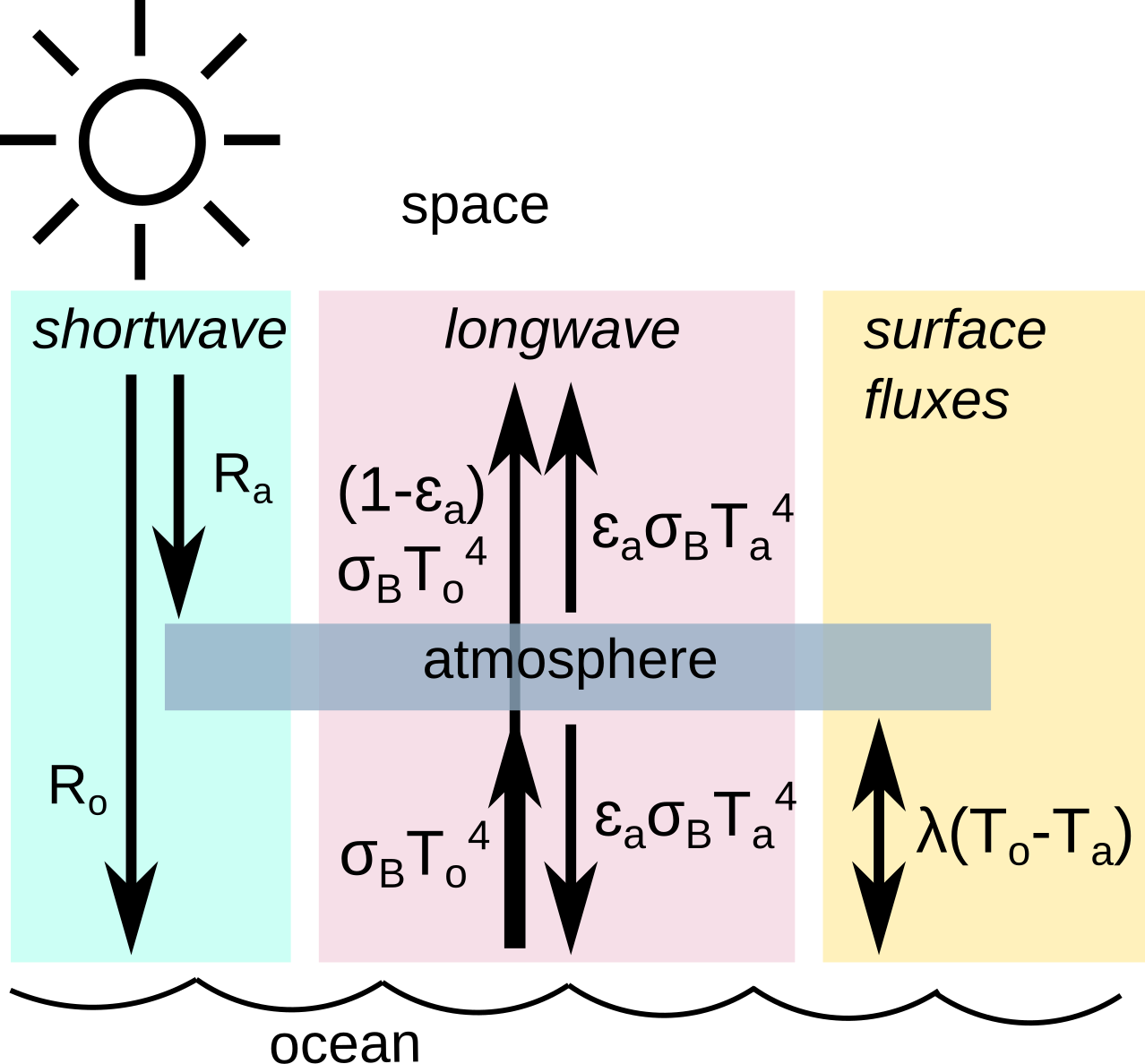
Sketch of the energy balance of [BB98]. It underlies the radiative and heat exchange scheme in the model.

../../_images/energybalance_detail.png

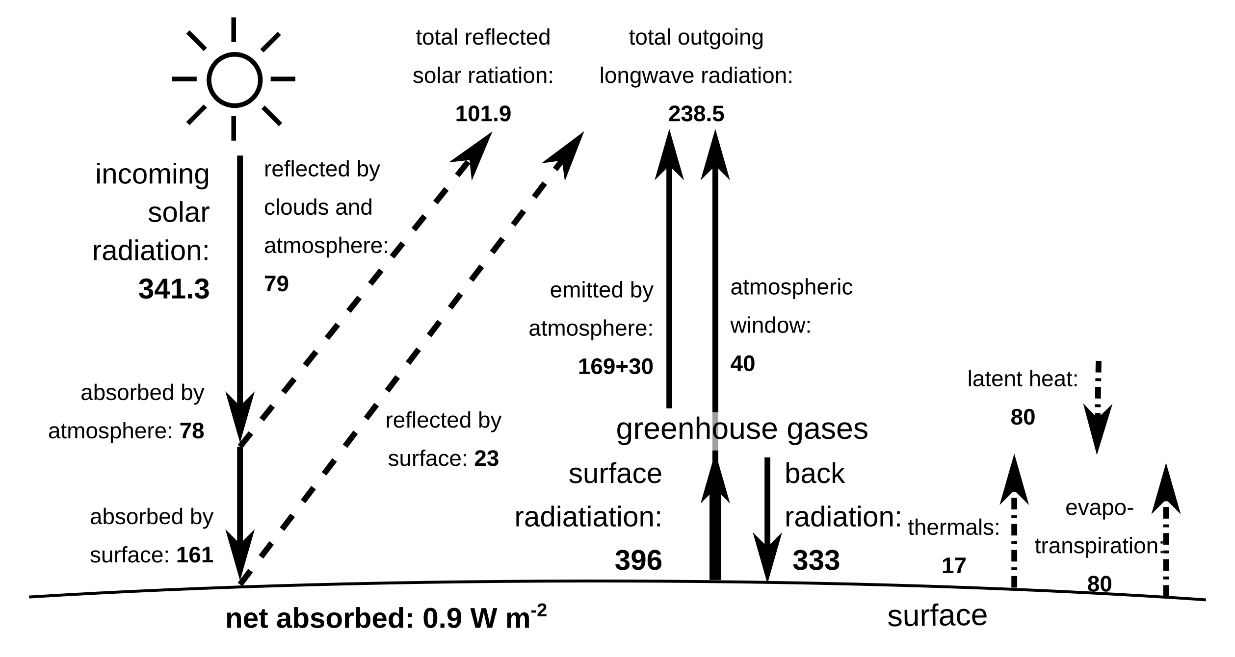
Actual values of the energy flux between the ground and the atmosphere [TFK09].

Set of basis functions

The present model solves the equations above by projecting them onto a basis of functions, to obtain a system of ordinary differential equations (ODE). This procedure is sometimes called a Galerkin expansion. This basis being finite, the resolution of the model is automatically truncated at the characteristic length of the highest-resolution function of the basis.

The atmospheric set of basis functions \(F_i\) is described in the section Projecting the equations on a set of basis functions.

The oceanic set of basis functions

Both oceanic fields \(\psi_{\rm o}\) and \(\delta T_{\rm o}\) are defined in a closed basin with no-flux boundary conditions (\(\partial \cdot_{\rm o} /\partial x \equiv 0\) at the meridional boundaries and \(\partial \cdot_{\rm o}/\partial y \equiv 0\) at the zonal boundaries).

These fields are projected on Fourier modes respecting these boundary conditions:

\[\phi_{H_{\rm o},P_{\rm o}} (x, y) = 2\sin(\frac{H_{\rm o} n}{2}x)\, \sin(P_{\rm o} y)\]

with integer values of \(H_{\rm o}\), \(P_{\rm o}\). Again, \(x\) and \(y\) are the horizontal adimensionalized coordinates defined above.

To easily manipulate these functions and the coefficients of the fields expansion, we number the basis functions along increasing values of \(H_{\rm o}\) and then \(P_{\rm o}\). It allows to write the set as \(\left\{ \phi_i(x,y); 1 \leq i \leq n_\text{o}\right\}\) where \(n_{\mathrm{o}}\) (nmod [1]) is the number of modes of the spectral expansion in the ocean.

For example, the model derived in [VDDCG15] can be specified by setting \(H_{\rm o} \in \{1,2\}\); \(P_{\rm o} \in \{1,4\}\) and the set of basis functions is

\[\begin{split}\phi_1(x,y) & = & 2\, \sin(\frac{n}{2} x)\, \sin(y), \nonumber \\ \phi_2(x,y) & = & 2\, \sin(\frac{n}{2} x)\, \sin(2 y), \nonumber \\ \phi_3(x,y) & = & 2\, \sin(\frac{n}{2} x)\, \sin(3 y), \nonumber \\ \phi_4(x,y) & = & 2\, \sin(\frac{n}{2} x)\, \sin(4 y), \nonumber \\ \phi_5(x,y) & = & 2\, \sin(n x)\, \sin(y), \nonumber \\ \phi_6(x,y) & = & 2\, \sin(n x)\, \sin(2 y), \nonumber \\ \phi_7(x,y) & = & 2\, \sin(n x)\, \sin(3 y), \nonumber \\ \phi_8(x,y) & = & 2\, \sin(n x)\, \sin(4 y), \nonumber\end{split}\]

such that

\[\nabla^2 \phi_i(x,y) = -m^2_i \,\phi_i(x,y)\]

with eigenvalues \(m_i^2 = P_{{\rm o},i}^2 + n^2 \, H_{{\rm o},i}^2/4\). These Fourier modes are also orthonormal with respect to the inner product

\[\frac{n}{2\pi^2}\int_0^\pi\int_0^{2\pi/n} \phi_i(x,y)\, \phi_j(x,y)\, \mathrm{d} x \, \mathrm{d} y = \delta_{ij}\]

where \(\delta_{ij}\) is the Kronecker delta. Note however that the atmospheric and oceanic basis \(F_i\) and \(\phi_i\) are not orthonormal to each other.

../../_images/visualise_basisfunctions_ocean.png

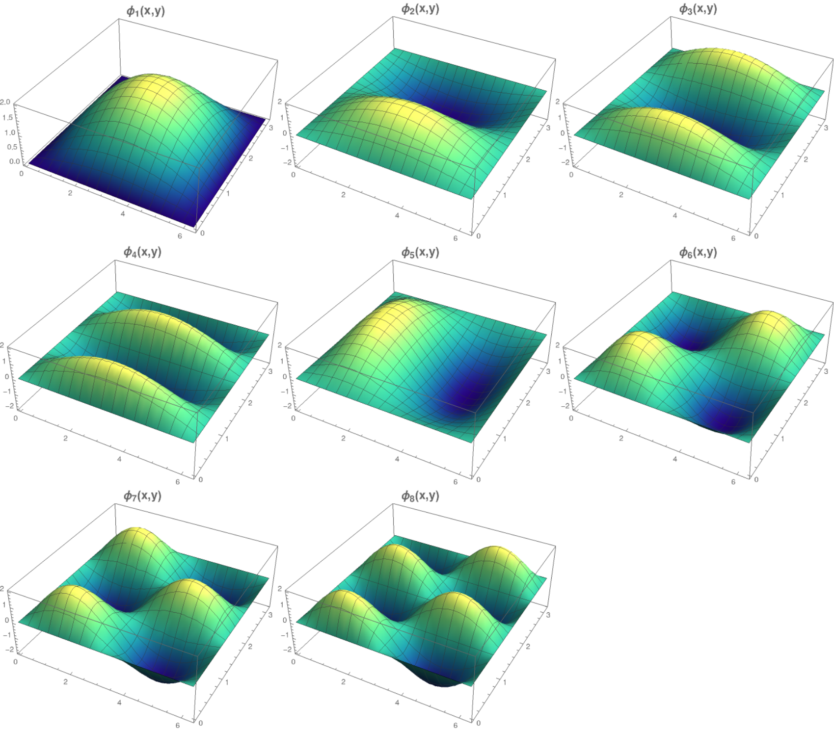
The first 8 basis functions \(\phi_i\) evaluated on the nondimensional domain of the model.

Fields expansion

The fields of the model can expanded on these sets of basis functions according to

\[\begin{split}\psi_\text{a} (x,y) &= \sum_{i=1}^{n_\text{a}} \; \psi_{\text{a},i} \, F_i(x,y), \\ \theta_\text{a}(x,y) &=\sum_{i=1}^{n_\text{a}} \theta_{\text{a},i} \; F_i(x,y), \\ \delta T_\text{a}(x,y) &=\sum_{i=1}^{n_\text{a}} \delta T_{\text{a},i} \; F_i(x,y), \\ &= 2 \frac{f_0}{R} \sum_{i=1}^{n_\text{a}} \theta_{\text{a},i} \; F_i(x,y), \nonumber\\ \psi_\text{o}(x,y) &= \sum_{j=1}^{n_\text{o}} \psi_{\text{o},j} \; (\phi_j(x,y) \; -\; \overline{\phi_j}), \\ \delta T_\text{o}(x,y) &= \sum_{j=1}^{n_\text{o}} \delta T_{\text{o},j} \; \phi_j(x,y).\end{split}\]

In the expansion for \(\psi_\text{o}\), a term \(\overline{\phi_j}\) is added to the oceanic basis function \(\phi_j\) in order to get a zero spatial average. This is required to guarantee mass conservation in the ocean, but otherwise does not affect the dynamics. Indeed, it can be added a posteriori when plotting the field \(\psi_\text{o}\). This term is non-zero for odd \(P_\text{o}\) and \(H_\text{o}\):

\[\begin{split}\overline{\phi_j} &= \frac{n}{2\pi^2} \int _0^{\pi }\int _0^{\frac{2 \pi }{n}}\phi_j(x,y) \,\text{d}x \,\text{d}y \\ &= 2\frac{((-1)^{H_\text{o}} - 1) ((-1)^{P_\text{o}} - 1)}{H_\text{o} P_\text{o} \pi^2}.\nonumber\end{split}\]

The mass conservation is automatically satisfied for \(\psi_\text{a}\), as the spatial averages of the atmospheric basis functions \(F_i\) are zero.

Furthermore, the short-wave radiation or insolation is determined by

\[\begin{split}\delta R_\text{a}(x,y) = \sum_{i=1}^{n_\text{a}} \, C_{\text{a},i} \, F_i, \\ \delta R_\text{o}(x,y) = \sum_{i=1}^{n_\text{a}} \, C_{\text{o},i} \, F_i.\end{split}\]

which we project on the same atmospheric basis of function to maintain consistency and allow meridional gradients. These decompositions are stored in the parameters AtmosphericTemperatureParams.C and OceanicTemperatureParams.C and can be set using the functions AtmosphericTemperatureParams.set_insolation and OceanicTemperatureParams.set_insolation.

The vertical velocity \(\omega(x,y)\) have also to be decomposed:

\[\omega(x,y) = \sum_{i=1}^{n_{\mathrm{a}}} \, \omega_i \, F_i(x,y) .\]

Ordinary differential equations

The fields, parameters and variables are non-dimensionalized by dividing time by \(f_0^{-1}\) (f0), distance by the characteristic length scale \(L\) (L), pressure by the difference \(\Delta p\) (deltap), temperature by \(f_0^2 L^2/R\), and streamfunction by \(L^2 f_0\). As a result of this non-dimensionalization, the fields \(\theta_{\rm a}\) and \(\delta T_{\rm a}\) can be identified: \(2 \theta_{\rm a} \equiv \delta T_{\rm a}\).

The ordinary differential equations of the truncated model are:

\[\begin{split}\dot\psi_{{\rm a},i} & = & - a_{i,i}^{-1} \sum_{j,m = 1}^{n_{\mathrm{a}}} b_{i, j, m} \left(\psi_{{\rm a},j}\, \psi_{{\rm a},m} + \theta_{{\rm a},j}\, \theta_{{\rm a},m}\right) - \beta\, a_{i,i}^{-1} \, \sum_{j=1}^{n_{\mathrm{a}}} \, c_{i, j} \, \psi_{{\rm a},j} \nonumber \\ & & \qquad \qquad \qquad \qquad - \frac{k_d}{2} \left(\psi_{{\rm a},i} - \theta_{{\rm a},i}\right) + \frac{k_d}{2} \, a_{i,i}^{-1} \, \sum_{j = 1}^{n_{\mathrm{o}}} d_{i,j} \, \psi_{{\rm o},j} \\ \dot\theta_{{\rm a},i} & = & - a_{i,i}^{-1} \sum_{j,m = 1}^{n_{\mathrm{a}}} b_{i, j, m} \left(\psi_{{\rm a},j}\, \theta_{{\rm a},m} + \theta_{{\rm a},j}\, \psi_{{\rm a},m}\right) - \beta\, a_{i,i}^{-1} \, \sum_{j=1}^{n_{\mathrm{a}}} \, c_{i, j} \, \theta_{{\rm a},j} \nonumber \\ & & \qquad \qquad \qquad \qquad + \frac{k_d}{2} \left(\psi_{{\rm a},i} - \theta_{{\rm a},i}\right) - \frac{k_d}{2} \, a_{i,i}^{-1} \, \sum_{j = 1}^{n_{\mathrm{o}}} d_{i,j} \, \psi_{{\rm o},j} - 2 \, k'_d \, \theta_{{\rm a},i} + a_{i,i}^{-1} \, \omega_i \\ \dot\theta_{\rm{a},i} & = & - \sum_{j,m = 1}^{n_{\mathrm{a}}} g_{i, j, m} \, \psi_{{\rm a},j}\, \theta_{{\rm a},m} + \frac{\sigma}{2}\, \omega_i - \left(\lambda'_{\rm a} + S_{B,{\rm a}} \right) \, \theta_{\rm{a},i} \nonumber \\ & & \qquad \qquad \qquad \qquad + \left(\frac{\lambda'_{\rm a}}{2}+ S_{B, {\rm o}}\right) \sum_{j=1}^{n_{\mathrm{o}}} \, s_{i, j} \, \delta T_{{\rm o},j} + C'_{\text{a},i} \\ \dot\psi_{{\rm o},i} & = & \frac{1}{\left(M_{i,i} + G\right)} \, \left\{ - \sum_{j,m = 1}^{n_{\mathrm{o}}} \, C_{i,j,k} \, \psi_{{\rm o},j} \, \psi_{{\rm o},k} - \beta \, \sum_{j = 1}^{n_{\mathrm{o}}} \, N_{i,j} \, \psi_{{\rm o}, j} - (d + r) \, \sum_{j = 1}^{n_{\mathrm{o}}} \, M_{i,j} \, \psi_{{\rm o},j} \right. \nonumber \\ & & \qquad \qquad \qquad \qquad + \left. d \, \sum_{j = 1}^{n_{\mathrm{a}}} \, K_{i,j} \, \left(\psi_{{\rm a}, j} - \theta_{{\rm a}, j}\right)\right\} \\ \dot\delta T_{{\rm o},i} & = & - \sum_{j,m = 1}^{n_{\mathrm{o}}} \, O_{i,j,m} \, \psi_{{\rm o},j} \, \delta T_{{\rm o},m} - \left(\lambda'_{\rm o}+ s_{B,{\rm o}}\right) \, \delta T_{{\rm o},i} + \left(2 \,\lambda'_{\rm o} + s_{B,{\rm a}}\right) \, \sum_{j=1}^{n_{\mathrm{a}}} \, W_{i,j} \, \theta_{{\rm a},j} + \sum_{j=1}^{n_{\mathrm{a}}} \, W_{i,j} \, C'_{{\rm o},j}\end{split}\]

where the parameters values have been replaced by their non-dimensional ones and we have also defined \(G = - L^2/L_R^2\) (G), \(\lambda'_{{\rm a}} = \lambda/(\gamma_{\rm a} f_0)\) (Lpa), \(\lambda'_{{\rm o}} = \lambda/(\gamma_{\rm o} f_0)\) (Lpgo), \(S_{B,{\rm a}} = 8\,\epsilon_{\rm a}\, \sigma_B \, T_{{\rm a},0}^3 / (\gamma_{\rm a} f_0)\) (LSBpa), \(S_{B,{\rm o}} = 2\,\epsilon_{\rm a}\, \sigma_B \, T_{{\rm a},0}^3 / (\gamma_{\rm a} f_0)\) (LSBpgo), \(s_{B,{\rm a}} = 8\,\epsilon_{\rm a}\, \sigma_B \, T_{{\rm a},0}^3 / (\gamma_{\rm o} f_0)\) (sbpa), \(s_{B,{\rm o}} = 4\,\sigma_B \, T_{{\rm a},0}^3 / (\gamma_{\rm o} f_0)\) (sbpgo), \(C'_{{\rm a},i} = R C_{{\rm a},i} / (2 \gamma_{\rm a} L^2 f_0^3)\) (Cpa), \(C'_{{\rm o},i} = R C_{{\rm o},i} / (\gamma_{\rm o} L^2 f_0^3)\) (Cpgo).

The coefficients \(a_{i,j}\), \(g_{i, j, m}\), \(b_{i, j, m}\) and \(c_{i, j}\) are the inner products of the Fourier modes \(F_i\):

\[\begin{split}a_{i,j} & = & \frac{n}{2\pi^2}\int_0^\pi\int_0^{2\pi/n} F_i(x,y)\, \nabla^2 F_j(x,y)\, \mathrm{d} x \, \mathrm{d} y = - \delta_{ij} \, a_i^2 \\ g_{i, j, m} & = & \frac{n}{2\pi^2}\int_0^\pi\int_0^{2\pi/n} F_i(x,y)\, J\left(F_j(x,y), F_m(x,y)\right) \, \mathrm{d} x \, \mathrm{d} y \\ b_{i, j, m} & = & \frac{n}{2\pi^2}\int_0^\pi\int_0^{2\pi/n} F_i(x,y)\, J\left(F_j(x,y), \nabla^2 F_m(x,y)\right) \, \mathrm{d} x \, \mathrm{d} y \\ c_{i, j} & = & \frac{n}{2\pi^2}\int_0^\pi\int_0^{2\pi/n} F_i(x,y)\, \frac{\partial}{\partial x} F_j(x,y) \, \mathrm{d} x \, \mathrm{d} y\end{split}\]

and the coefficients \(M_{i,j}\), \(O_{i, j, m}\), \(C_{i, j, m}\) and \(N_{i, j}\) are the inner products of the Fourier modes \(\phi_i\):

\[\begin{split}M_{i,j} & = & \frac{n}{2\pi^2}\int_0^\pi\int_0^{2\pi/n} \phi_i(x,y)\, \nabla^2 \phi_j(x,y)\, \mathrm{d} x \, \mathrm{d} y = - \delta_{ij} \, m_i^2 \\ O_{i, j, m} & = & \frac{n}{2\pi^2}\int_0^\pi\int_0^{2\pi/n} \phi_i(x,y)\, J\left(\phi_j(x,y), \phi_m(x,y)\right) \, \mathrm{d} x \, \mathrm{d} y \\ C_{i, j, m} & = & \frac{n}{2\pi^2}\int_0^\pi\int_0^{2\pi/n} \phi_i(x,y)\, J\left(\phi_j(x,y), \nabla^2 \phi_m(x,y)\right) \, \mathrm{d} x \, \mathrm{d} y \\ N_{i, j} & = & \frac{n}{2\pi^2}\int_0^\pi\int_0^{2\pi/n} \phi_i(x,y)\, \frac{\partial}{\partial x} \phi_j(x,y) \, \mathrm{d} x \, \mathrm{d} y.\end{split}\]

The coefficients involved in the ocean-atmosphere interactions \(W_{i,j}\), \(K_{i, j}\), \(d_{i, j}\) and \(s_{i, j}\) are the inner products between the Fourier modes \(\phi_i\) and \(F_i\):

\[\begin{split}d_{i,j} & = & \frac{n}{2\pi^2}\int_0^\pi\int_0^{2\pi/n} F_i(x,y)\, \nabla^2 \phi_j(x,y)\, \mathrm{d} x \, \mathrm{d} y \\ K_{i,j} & = & \frac{n}{2\pi^2}\int_0^\pi\int_0^{2\pi/n} \phi_i(x,y)\, \nabla^2 F_j(x,y)\, \mathrm{d} x \, \mathrm{d} y \\ W_{i, j} & = & \frac{n}{2\pi^2}\int_0^\pi\int_0^{2\pi/n} \phi_i(x,y)\, F_j(x,y) \, \mathrm{d} x \, \mathrm{d} y = s_{j, i}\end{split}\]

These inner products are computed according to formulas detailed in [DCDV16] and stored in objects derived from the AtmosphericInnerProducts and OceanicInnerProducts classes.

The vertical velocity \(\omega_i\) can be eliminated, leading to the final equations

\[\begin{split}\dot\psi_{{\rm a},i} & = & - a_{i,i}^{-1} \sum_{j,m = 1}^{n_{\mathrm{a}}} b_{i, j, m} \left(\psi_{{\rm a},j}\, \psi_{{\rm a},m} + \theta_{{\rm a},j}\, \theta_{{\rm a},m}\right) - \beta\, a_{i,i}^{-1} \, \sum_{j=1}^{n_{\mathrm{a}}} \, c_{i, j} \, \psi_{{\rm a},j} \nonumber \\ & & \qquad \qquad \qquad \qquad - \frac{k_d}{2} \left(\psi_{{\rm a},i} - \theta_{{\rm a},i}\right) + \frac{k_d}{2} \, a_{i,i}^{-1} \, \sum_{j = 1}^{n_{\mathrm{o}}} d_{i,j} \, \psi_{{\rm o},j} \\ \dot\theta_{{\rm a},i} & = & \frac{\sigma/2}{a_{i,i} \,\sigma/2 - 1} \left\{ - \sum_{j,m = 1}^{n_{\mathrm{a}}} b_{i, j, m} \left(\psi_{{\rm a},j}\, \theta_{{\rm a},m} + \theta_{{\rm a},j}\, \psi_{{\rm a},m}\right) - \beta\, \, \sum_{j=1}^{n_{\mathrm{a}}} \, c_{i, j} \, \theta_{{\rm a},j} \right. \nonumber \\ & & \qquad \qquad \qquad \qquad + \left. \frac{k_d}{2} \, a_{i,i} \left(\psi_{{\rm a},i} - \theta_{{\rm a},i}\right) - \frac{k_d}{2} \, \sum_{j = 1}^{n_{\mathrm{o}}} d_{i,j} \, \psi_{{\rm o},j} -2 \, k'_d \, a_{i,i} \, \theta_{{\rm a},i} \right\} \nonumber \\ & & + \frac{1}{a_{i,i} \,\sigma/2 - 1} \left\{ \sum_{j,m = 1}^{n_{\mathrm{a}}} g_{i, j, m} \, \psi_{{\rm a},j}\, \theta_{{\rm a},m} + \left(\lambda'_{\rm a} + S_{B,{\rm a}} \right) \, \theta_{\rm{a},i} \right. \nonumber \\ & & \qquad \qquad \qquad \qquad - \left.\left(\frac{\lambda'_{\rm a}}{2}+ S_{B, {\rm o}}\right) \sum_{j=1}^{n_{\mathrm{o}}} \, s_{i, j} \, \delta T_{{\rm o},j} - C'_{\text{a},i} \right\} \\ \dot\psi_{{\rm o},i} & = & \frac{1}{\left(M_{i,i} + G\right)} \, \left\{ - \sum_{j,m = 1}^{n_{\mathrm{o}}} \, C_{i,j,k} \, \psi_{{\rm o},j} \, \psi_{{\rm o},k} - \beta \, \sum_{j = 1}^{n_{\mathrm{o}}} \, N_{i,j} \, \psi_{{\rm o}, j} - (d + r) \, \sum_{j = 1}^{n_{\mathrm{o}}} \, M_{i,j} \, \psi_{{\rm o},j} \right. \nonumber \\ & & \qquad \qquad \qquad \qquad + \left. d \, \sum_{j = 1}^{n_{\mathrm{a}}} \, K_{i,j} \, \left(\psi_{{\rm a}, j} - \theta_{{\rm a}, j}\right)\right\} \\ \dot\delta T_{{\rm o},i} & = & - \sum_{j,m = 1}^{n_{\mathrm{o}}} \, O_{i,j,m} \, \psi_{{\rm o},j} \, \delta T_{{\rm o},m} - \left(\lambda'_{\rm o}+ s_{B,{\rm o}}\right) \, \delta T_{{\rm o},i} + \left(2 \,\lambda'_{\rm o} + s_{B,{\rm a}}\right) \, \sum_{j=1}^{n_{\mathrm{a}}} \, W_{i,j} \, \theta_{{\rm a},j} + \sum_{j=1}^{n_{\mathrm{a}}} \, W_{i,j} \, C'_{{\rm o},j}\end{split}\]

that are implemented by means of a tensorial contraction:

\[\frac{\text{d}\eta_i}{\text{d}t} = \sum_{j, k=0}^{2 (n_\mathrm{a}+n_\mathrm{o})} \mathcal{T}_{i,j,k} \; \eta_j \; \eta_k\]

with \(\boldsymbol{\eta} = (1, \psi_{{\rm a},1}, \ldots, \psi_{{\rm a},n_\mathrm{a}}, \theta_{{\rm a},1}, \ldots, \theta_{{\rm a},n_\mathrm{a}}, \psi_{{\rm o},1}, \ldots, \psi_{{\rm o},n_\mathrm{o}}, \delta T_{{\rm o},1}, \ldots, \delta T_{{\rm o},n_\mathrm{o}})\), as described in the Code Description. Note that \(\eta_0 \equiv 1\). The tensor \(\mathcal{T}\), which fully encodes the bilinear system of ODEs above, is computed and stored in the QgsTensor.

Example

An example about how to setup the model to use this model version is shown in Recovering the result of De Cruz, Demaeyer and Vannitsem (2016).

MAOSOAM model version

qgs allows one to specify the basis of functions over which the PDE equations of the model are projected. Therefore it is easy to reproduce the model proposed in [VSolePDC19], where the atmosphere and the ocean are subject to the same periodic channel boundary conditions.

../../_images/model_variables_maosoam_duck.png

Sketch of the ocean-atmosphere coupled model layers for the MAOSOAM model version, where both the atmosphere and the ocean are periodic channels. The domain (\(\beta\)-plane) zonal and meridional coordinates are labeled as the \(x\) and \(y\) variables.

The basis of functions in the ocean is thus defined as:

\[\begin{split}\begin{aligned} \phi_{1}(x, y)&= F_{1} (x, y) = \sqrt{2}\cos(y),\\ \phi_{2}(x, y)&= F_{2} (x, y) = 2 \cos (n x) \sin (y),\\ &\vdots \end{aligned}\end{split}\]

while the basis of functions is the same between the atmosphere and ocean.

Since these boundary conditions mimick the situation in the southern hemisphere, this model is called the Modular Arbitrary-Order Southern Ocean-Atmosphere Model (MAOSOAM). This change in basis does not alter the ordinary differential equations shown above.

An example of how to setup this model version is given in Recovering the result of Vannitsem, Solé-Pomies and De Cruz (2019).

Dynamical temperatures and quartic temperature tendencies model version

It is possible to calculate solutions of the model without linearizing the quartic long-wave radiation terms of the temperature equations for \(T_\text{a}\) and \(T_\text{o}\). Instead, these radiation terms can be expanded onto the set of basis functions, including the 0-th order reference temperatures \(T_{\text{a}, 0}\) and \(T_{\text{o}, 0}\).

This requires the introduction of a new basis function, which is the constant basis: ‘\(1\)’. Thus the atmospheric and oceanic basis functions are now expanded as follow:

\[\begin{split}\begin{aligned} \phi_0(x, y)&=1,\\ \phi_{1}(x, y)&=2 \sin \left(\frac{n}{2} x\right) \sin (y),\\ \phi_{2}(x, y)&=2 \sin (n x) \sin (y),\\ &\vdots \end{aligned} \qquad \begin{aligned} F_0(x, y)&=1,\\ F_{1}(x, y)&=\sqrt{2}\cos(y),\\ F_{2}(x, y)&=2 \cos (n x) \sin (y),\\ &\vdots \end{aligned}\end{split}\]

The temperature fields are then expanded onto these functions:

\[T_\text{o}(x, y)=\sum_{j=0}^{n_\text{o}}T_{\text{o}, j}\,\phi_j(x, y)\qquad T_\text{a}(x, y)=\sum_{j=0}^{n_\text{a}}T_{\text{a}, j}\, F_j(x, y) = T_{\text{a}, 0} \, F_0(x, y) + 2 \frac{f_{0}}{R} \sum_{i=1}^{n_{\mathrm{a}}} \theta_{\mathrm{a}, i} F_{i}(x, y) .\]

Likewise, the short-wave radiation fluxes are expanded as

\[R_\text{o}=R_{\text{o}, 0} + \delta R_\text{o} = \sum_{j=0}^{n_\text{o}}C_{\text{o}, j}\, F_j(x, y)\qquad R_\text{a}=R_{\text{a}, 0} + \delta R_\text{a} = \sum_{j=0}^{n_\text{a}}C_{\text{a}, j}\, F_j(x, y),\]

where we are thus identifying \(R_{\text{o}, 0}=C_{\text{o}, 0}\) and \(R_{\text{a}, 0}=C_{\text{a}, 0}\).

Consequences in the ocean

This modified expansion involves re-writing the ocean temperature equations as:

\[\begin{split}&\gamma_{\mathrm{o}}\Bigg(\frac{\partial }{\partial t} \sum_{j=0}^{n_\text{o}}T_{\text{o}, j}\,\phi_j(x, y)+J\left(\sum_{m=1}^{n_\text{o}} \psi_{\mathrm{o}, m}\,\phi_m(x, y), \sum_{j=0}^{n_\text{o}}T_{\text{o}, j}\,\phi_j(x, y)\right) \Bigg)=\\ &\qquad \qquad \qquad \qquad -\lambda\left(\sum_{j=0}^{n_\text{o}}T_{\text{o}, j}\,\phi_j(x, y)-\sum_{j=0}^{n_\text{a}}T_{\text{a}, j}\,F_j(x, y)\right)\\ &\qquad \qquad \qquad \qquad -\sigma_{B} \left(\sum_{j=0}^{n_\text{o}}T_{\text{o}, j}\,\phi_j(x, y)\right)^{4} +\epsilon_{\mathrm{a}} \sigma_{B} \left(\sum_{j=0}^{n_\text{a}}T_{\text{a}, j}\, F_j(x, y)\right)^4+R_{\mathrm{o}}\end{split}\]

This equation is then simplified and non-dimensionalized as in the linearized case. This leads to the ordinary differential equation for the ocean temperature with quartic terms:

\[\begin{split}&\sum_{j=0}^{n_\text{o}}U_{i, j}\,\dot{T}_{\text{o}, j}= -\sum_{j,k=1}^{n_\text{o}}O_{i,j,m}\,\psi_{\text{o}, j}\,T_{\text{o}, m} -\sum_{j=0}^{n_\text{o}}\lambda'_\text{o}\, U_{i,j}T_{\text{o}, j}\\ &\qquad \qquad \qquad -s_{B, \text{o}}\sum_{j,k,l,m=0}^{n_\text{o}}V_{i,j,k,l,m}\, T_{\text{o}, j}T_{\text{o},k}T_{\text{o},l}T_{\text{o},m}+2\lambda_\text{o}'\sum_{j=0}^{n_\text{a}}W_{i,j}\,\theta_{\text{a},j}\\ &\qquad \qquad \qquad +s_{B, \text{a}} \sum_{j,k,l,m=0}^{n_\text{a}}Z_{i,j,k,l,m}\,\theta_{\text{a},j}\theta_{\text{a},k}\theta_{\text{a},l}\theta_{\text{a},m} +\sum_{j=0}^{n_\text{o}}W_{i,j}\, C'_{\text{o},j}\end{split}\]

where here \(s_{B,\text{o}}=\sigma_B f_0^5 L^6/(\gamma_\text{o} R^3)\) (T4sbpgo), and \(s_{B, \text{a}}=16 \varepsilon_\text{a} \sigma_B f_0^5 L^6/(\gamma_\text{o} R^3)\) (T4sbpa).

The coefficients \(U_{i, j}\), \(V_{i,j,k,l,m}\), and \(Z_{i,j,k,l,m}\) are the inner products of the basis functions \(\phi_{i}\) and are defined as:

\[U_{i, j}=\frac{n}{2 \pi^{2}} \int_{0}^{\pi} \int_{0}^{2 \pi / n} \phi_{i}(x, y)~\phi_{j}(x, y)\, \mathrm{d} x \, \mathrm{d} y\]
\[V_{i, j, k, l, m}=\frac{n}{2 \pi^{2}} \int_{0}^{\pi} \int_{0}^{2 \pi / n} \phi_{i}(x, y)~\phi_{j}(x, y)~\phi_{k}(x, y)~\phi_{l}(x, y)~\phi_{m}(x, y)\, \mathrm{d} x \, \mathrm{d} y\]
\[Z_{i, j, k, l, m}=\frac{n}{2 \pi^{2}} \int_{0}^{\pi} \int_{0}^{2 \pi / n} \phi_{i}(x, y)~F_{j}(x, y)~F_{k}(x, y)~F_{l}(x, y)~F_{m}(x, y)\, \mathrm{d} x \, \mathrm{d} y,\]

These inner products are stored in objects derived from the OceanicInnerProducts classes.

The equation corresponding to the oceanic barotropic streamfunction \(\psi_\text{o}(x, y)=\sum_{j=1}^{n_\text{o}}\psi_{\text{o}, j}\, \phi_j(x, y)\) is unchanged by the modified expansion and is given by:

\[\begin{split}\sum_{j=1}^{n_\text{o}} \left(M_{i,j} + G\, U_{i,j}\right) \dot\psi_{{\rm o},j} & = & - \sum_{j,m = 1}^{n_{\mathrm{o}}} \, C_{i,j,k} \, \psi_{{\rm o},j} \, \psi_{{\rm o},k} - \beta \, \sum_{j = 1}^{n_{\mathrm{o}}} \, N_{i,j} \, \psi_{{\rm o}, j} - (d + r) \, \sum_{j = 1}^{n_{\mathrm{o}}} \, M_{i,j} \, \psi_{{\rm o},j} \nonumber \\ & & \qquad \qquad \qquad \qquad + d \, \sum_{j = 1}^{n_{\mathrm{a}}} \, K_{i,j} \, \left(\psi_{{\rm a}, j} - \theta_{{\rm a}, j}\right) \\\end{split}\]

Consequences in the atmosphere

The atmosphere temperature equation now reads:

\[\begin{split}&\gamma_{\mathrm{a}}\left(\frac{\partial}{\partial t}\sum_{j=0}^{n_\text{a}}T_{\text{a}, j}\, F_j(x, y)+J\left(\sum_{m=1}^{n_\text{a}} \psi_{\mathrm{a}, m}\, F_m(x, y), \sum_{j=0}^{n_\text{a}}T_{\text{a}, j}\,F_j(x, y)\right)-\sigma \omega \frac{p}{R}\right)=\\ &\qquad \qquad \qquad \qquad -\lambda\left(\sum_{j=0}^{n_\text{a}}T_{\text{a}, j}\, F_j(x, y)-\sum_{j=0}^{n_\text{o}}T_{\text{o}, j}\,\phi_j(x, y)\right)\\ &\qquad \qquad \qquad \qquad +\epsilon_{\mathrm{a}} \sigma_{B} \left(\sum_{j=0}^{n_\text{o}}T_{\text{o}, j}\,\phi_j(x, y)\right)^4-2 \epsilon_{\mathrm{a}} \sigma_{B} \left(\sum_{j=0}^{n_\text{a}}T_{\text{a}, j}\, F_j(x, y)\right)^4+R_{\mathrm{a}}.\end{split}\]

The atmospheric baroclinic streamfunction is calculated in a similar manner to the ocean temperature equation, where the identity \(T_{\text{a}, 0} \equiv 2 \frac{f_{0}}{R} \theta_{\mathrm{a}, 0}\) is used:

\[\begin{split}&\sum_{j=0}^{n_\text{a}}u_{i, j}\,\dot{\theta}_{\text{a}, j}= -\sum_{j,k=1}^{n_\text{a}}g_{i,j,m}\,\psi_{\text{a}, j}\,\theta_{\text{a}, m}+\frac{\sigma}{2}\sum_{j=1}^{n_\text{a}}u_{i,j}\,\omega_j-\lambda'_\text{a}\sum_{j=0}^{n_\text{a}}u_{i,j}\,\theta_{\text{a}, j}\\ &\qquad \qquad \qquad -S_{B,\text{a}}\sum_{j,k,l,m=0}^{n_\text{a}}z_{i,j,k,l,m}\,\theta_{\text{a}, j}\theta_{\text{a},k}\theta_{\text{a},l}\theta_{\text{a},m}+\frac{\lambda'_\text{a}}{2}\sum_{j=0}^{n_\text{o}}s_{i,j}\, T_{\text{o}, j}\\ &\qquad \qquad \qquad +S_{B, \text{o}}\sum_{j,k,l,m=0}^{n_\text{o}}v_{i,j,k,l,m}\, T_{\text{o}, j}T_{\text{o},k}T_{\text{o},l}T_{\text{o},m}+\sum_{j=0}^{n_\text{a}}u_{i,j}\, C'_{\text{a},j}\end{split}\]

where \(S_{B,\text{a}}=16\varepsilon_\text{a}\sigma_B L^6 f_0^5/(\gamma_\text{a}R^3)\) (T4LSBpa) and \(S_{B, \text{o}}=\varepsilon_\text{a} \sigma_B L^6 f_0^5/(2\gamma_\text{a}R)\) (T4LSBpgo).

The coefficients \(u_{i, j}\), \(v_{i,j,k,l,m}\), and \(z_{i,j,k,l,m}\) are the corresponding inner products of the basis functions \(F_{i}\):

\[u_{i, j}=\frac{n}{2 \pi^{2}} \int_{0}^{\pi} \int_{0}^{2 \pi / n} F_{i}(x, y)~F_{j}(x, y)\, \mathrm{d} x \mathrm{~d} y\]
\[v_{i, j, k, l, m}=\frac{n}{2 \pi^{2}} \int_{0}^{\pi} \int_{0}^{2 \pi / n} F_{i}(x, y)~\phi_{j}(x, y)~\phi_{k}(x, y)~\phi_{l}(x, y)~\phi_{m}(x, y)\, \mathrm{d} x \mathrm{~d} y\]
\[z_{i, j, k, l, m}=\frac{n}{2 \pi^{2}} \int_{0}^{\pi} \int_{0}^{2 \pi / n} F_{i}(x, y)~F_{j}(x, y)~F_{k}(x, y)~F_{l}(x, y)~F_{m}(x, y)\, \mathrm{d} x \mathrm{~d} y\]

These inner products are stored in objects derived from the AtmosphericInnerProducts.

Besides the two equations for the temperatures, the equations for the atmospheric barotropic and the baroclinic streamfunctions:

\[\psi_\text{a}(x, y)=\sum_{j=1}^{n_\text{a}}\psi_{\text{a}, j}\, F_j(x, y)\qquad \theta_\text{a}(x, y)=\sum_{j=1}^{n_\text{a}} \theta_{\text{a}, j}\, F_j(x, y),\]

derived in the linearized case are still valid here:

\[\begin{split}\sum_{j=1}^{n_\text{a}} a_{i,j} \, \dot\psi_{{\rm a},j} & = & - \sum_{j,m = 1}^{n_{\mathrm{a}}} b_{i, j, m} \left(\psi_{{\rm a},j}\, \psi_{{\rm a},m} + \theta_{{\rm a},j}\, \theta_{{\rm a},m}\right) - \beta\, \sum_{j=1}^{n_{\mathrm{a}}} \, c_{i, j} \, \psi_{{\rm a},j} \nonumber \\ & & \qquad \qquad \qquad \qquad - \frac{k_d}{2} \sum_{j=1}^{n_\text{a}} a_{i,j} \left(\psi_{{\rm a},j} - \theta_{{\rm a},j}\right) + \frac{k_d}{2} \, \sum_{j = 1}^{n_{\mathrm{o}}} d_{i,j} \, \psi_{{\rm o},j} \\ \sum_{j=1}^{n_\text{a}} a_{i,j} \, \dot\theta_{{\rm a},j} & = & - \sum_{j,m = 1}^{n_{\mathrm{a}}} b_{i, j, m} \left(\psi_{{\rm a},j}\, \theta_{{\rm a},m} + \theta_{{\rm a},j}\, \psi_{{\rm a},m}\right) - \beta\, \sum_{j=1}^{n_{\mathrm{a}}} \, c_{i, j} \, \theta_{{\rm a},j} \nonumber \\ & & \qquad \qquad \qquad \qquad + \frac{k_d}{2} \sum_{j=1}^{n_\text{a}} a_{i,j} \left(\psi_{{\rm a},j} - \theta_{{\rm a},j}\right) - \frac{k_d}{2} \, \sum_{j = 1}^{n_{\mathrm{o}}} d_{i,j} \, \psi_{{\rm o},j} \nonumber \\ & & \qquad \qquad \qquad \qquad - 2 \, k'_d \, \sum_{j=1}^{n_\text{a}} a_{i,j} \, \theta_{{\rm a},j} + \sum_{j=1}^{n_\text{a}} u_{i,j} \, \omega_j \\\end{split}\]

As with the MAOOAM model with linearized temperature described above, the vertical velocity is then eliminated to provide a single equation for the atmospheric baroclinic streamfunction. The resulting closed baroclinic streamfunction equation, with \(T_{\text{a}, 0} \equiv 2 \frac{f_{0}}{R} \theta_{\mathrm{a}, 0}\), is:

\[\begin{split}\frac{\sigma}{2}\sum_{j=1}^{n_\text{a}} a_{i, j}~\dot{\theta}_{\text{a}, j} - \sum_{j=0}^{n_\text{a}} u_{i, j}~\dot{\theta}_{\text{a}, j}&=\frac{\sigma}{2}\bigg\{- \sum_{j,m = 1}^{n_{\mathrm{a}}} b_{i, j, m} \left(\psi_{{\rm a},j}\, \theta_{{\rm a},m} + \theta_{{\rm a},j}\, \psi_{{\rm a},m}\right) - \beta\, \sum_{j=1}^{n_{\mathrm{a}}} \, c_{i, j} \, \theta_{{\rm a},j} \\ & + \frac{k_d}{2} \sum_{j=1}^{n_\text{a}} a_{i,j} \left(\psi_{{\rm a},j} - \theta_{{\rm a},j}\right) - \frac{k_d}{2} \, \sum_{j = 1}^{n_{\mathrm{o}}} d_{i,j} \, \psi_{{\rm o},j} - 2 \, k'_d \, \sum_{j=1}^{n_\text{a}} a_{i,j} \, \theta_{{\rm a},j} \bigg\} \\ &+\bigg\{\sum_{j,k=1}^{n_\text{a}}g_{i,j,m}\,\psi_{\text{a}, j}\,\theta_{\text{a}, m}+\lambda'_\text{a}\sum_{j=0}^{n_\text{a}}u_{i,j}\,\theta_{\text{a}, j}\\ &+S_{B,\text{a}}\sum_{j,k,l,m=0}^{n_\text{a}}z_{i,j,k,l,m}\,\theta_{\text{a}, j}\theta_{\text{a},k}\theta_{\text{a},l}\theta_{\text{a},m}-\frac{\lambda'_\text{a}}{2}\sum_{j=0}^{n_\text{o}}s_{i,j}\, T_{\text{o}, j}\\ &-S_{B, \text{o}}\sum_{j,k,l,m=0}^{n_\text{o}}v_{i,j,k,l,m}\, T_{\text{o}, j}T_{\text{o},k}T_{\text{o},l}T_{\text{o},m}-\sum_{j=0}^{n_\text{a}}u_{i,j}\, C'_{\text{a},j}\bigg\}\end{split}\]

These equations are implemented by means of a tensor contraction:

\[\frac{\mathrm{d} \eta_{i}}{\mathrm{d} t}=\sum_{j, k, l, m, n=0}^{2\left(n_{\mathrm{a}}+n_{\mathrm{o}}+1\right)} \mathcal{T}_{i, j, k, l, m} \,\eta_{j} \eta_{k}\eta_{l}\eta_{m}\]

with \(\eta=(1, \psi_{\text{a},1},\dots,\psi_{\text{a},n_\text{a}},\theta_{\text{a}, 0},\theta_{\text{a}, 1},\dots,\theta_{\text{a}, n_\text{a}},\psi_{\text{o}, 1},\dots,\psi_{\text{o}, n_o},T_{o, 0},T_{\text{o}, 1},\dots,T_{\text{o}, n_o})\), which is described in more detail in the Code Description page, see in particular the section Special case with the quartic temperature scheme. This specific temperature scheme can be activated by setting the parameter QgParams.T4 to True when instantiating the model’s QgParams parameters object.

Dynamical temperature and linearized temperature tendencies model version

As an alternative to the quartic temperature tendencies, it is also possible to use dynamic zero-th order reference temperatures while preserving the linearization of the temperature perturbations. This differs from the linearised version of the model, described in the section Temperature equations, as here the reference temperatures \(T_{{\rm o}, 0}\) and \(T_{{\rm a}, 0}\) are considered as spatially uniform but not constant in time. These temperatures are therefore calculated at every time step.

In this version, the radiative quartic terms in the equations described in the previous section are linearized by setting the indices \(j, k\) and \(l\) to zero, hence dropping the higher-order dependencies in the perturbations. The linearized ocean temperature equation is reduced to the following equation:

\[\begin{split}&\sum_{j=0}^{n_\text{o}}U_{i, j}\,\dot{T}_{\text{o}, j}= -\sum_{j,k=1}^{n_\text{o}}O_{i,j,m}\,\psi_{\text{o}, j}\,T_{\text{o}, m} -\sum_{j=0}^{n_\text{o}}\lambda'_\text{o}\, U_{i,j}T_{\text{o}, j}\\ &\qquad \qquad \qquad - 4 \, s_{B, \text{o}}\sum_{m=0}^{n_\text{o}}V_{i,0,0,0,m}\, T_{\text{o}, 0}^3\, T_{\text{o},m}+2\lambda_\text{o}'\sum_{j=0}^{n_\text{a}}W_{i,j}\,\theta_{\text{a},j}\\ &\qquad \qquad \qquad + 4 \, s_{B, \text{a}} \sum_{m=0}^{n_\text{a}}Z_{i,0,0,0,m}\,\theta_{\text{a},0}^3\,\theta_{\text{a},m} +\sum_{j=0}^{n_\text{o}}W_{i,j}\, C'_{\text{o},j} ,\end{split}\]

and similarly for the atmospheric temperature:

\[\begin{split}\frac{\sigma}{2}\sum_{j=1}^{n_\text{a}} a_{i, j}~\dot{\theta}_{\text{a}, j} - \sum_{j=0}^{n_\text{a}} u_{i, j}~\dot{\theta}_{\text{a}, j}&=\frac{\sigma}{2}\bigg\{- \sum_{j,m = 1}^{n_{\mathrm{a}}} b_{i, j, m} \left(\psi_{{\rm a},j}\, \theta_{{\rm a},m} + \theta_{{\rm a},j}\, \psi_{{\rm a},m}\right) - \beta\, \sum_{j=1}^{n_{\mathrm{a}}} \, c_{i, j} \, \theta_{{\rm a},j} \\ & + \frac{k_d}{2} \sum_{j=1}^{n_\text{a}} a_{i,j} \left(\psi_{{\rm a},j} - \theta_{{\rm a},j}\right) - \frac{k_d}{2} \, \sum_{j = 1}^{n_{\mathrm{o}}} d_{i,j} \, \psi_{{\rm o},j} - 2 \, k'_d \, \sum_{j=1}^{n_\text{a}} a_{i,j} \, \theta_{{\rm a},j} \bigg\} \\ &+\bigg\{\sum_{j,k=1}^{n_\text{a}}g_{i,j,m}\,\psi_{\text{a}, j}\,\theta_{\text{a}, m}+\lambda'_\text{a}\sum_{j=0}^{n_\text{a}}u_{i,j}\,\theta_{\text{a}, j}\\ &+ 4 \, S_{B,\text{a}}\sum_{m=0}^{n_\text{a}}z_{i,0,0,0,m}\,\theta_{\text{a},0}^3\,\theta_{\text{a}, m}-\frac{\lambda'_\text{a}}{2}\sum_{j=0}^{n_\text{o}}s_{i,j}\, T_{\text{o}, j}\\ &- 4 \, S_{B, \text{o}}\sum_{m=0}^{n_\text{o}}v_{i,0,0,0,m}\, T_{\text{o}, 0}^3\, T_{\text{o},m}-\sum_{j=0}^{n_\text{a}}u_{i,j}\, C'_{\text{a},j}\bigg\}.\end{split}\]

On the other hand, the equations for \(\psi_{\rm a}\) and \(\psi_{\rm o}\) are unchanged. This particular temperature scheme can be activated by setting the parameter QgParams.dynamic_T to True when instantiating the model’s QgParams parameters object.

References

BB98(1,2)

J. J. Barsugli and D. S. Battisti. The basic effects of atmosphere-ocean thermal coupling on midlatitude variability*. Journal of the Atmospheric Sciences, 55(4):477–493, 1998. URL: https://journals.ametsoc.org/doi/full/10.1175/1520-0469%281998%29055%3C0477%3ATBEOAO%3E2.0.CO%3B2.

DCDV16

L. De Cruz, J. Demaeyer, and S. Vannitsem. The Modular Arbitrary-Order Ocean-Atmosphere Model: MAOOAM v1.0. Geoscientific Model Development, 9(8):2793–2808, 2016. URL: https://www.geosci-model-dev.net/9/2793/2016/.

TFK09

K. E. Trenberth, J. T. Fasullo, and J. Kiehl. Earth's global energy budget. Bulletin of the American Meteorological Society, 90(3):311–324, 2009.

VDDCG15(1,2)

S. Vannitsem, J. Demaeyer, L. De Cruz, and M. Ghil. Low-frequency variability and heat transport in a low-order nonlinear coupled ocean–atmosphere model. Physica D: Nonlinear Phenomena, 309:71–85, 2015. URL: https://www.sciencedirect.com/science/article/abs/pii/S0167278915001335.

VSolePDC19

Stéphane Vannitsem, Roman Solé-Pomies, and Lesley De Cruz. Routes to long-term atmospheric predictability in reduced-order coupled ocean–atmosphere systems: impact of the ocean basin boundary conditions. Quarterly Journal of the Royal Meteorological Society, 145(723):2791–2805, 2019. URL: https://doi.org/10.1002/qj.3594.