Recovering the result of Vannitsem, Solé-Pomies and De Cruz (2019)
In this example, we recover the attractor shown in
Vannitsem, S., Solé‐Pomies, R. and De Cruz, L. (2019). Routes to long‐term atmospheric predictability in reduced‐order coupled ocean–atmosphere systems ‐ Impact of the ocean basin boundary conditions. Quarterly Journal of the Royal Meteorological Society, 145: 2791– 2805. doi.org/10.1002/qj.3594
obtained with a 2-layer channel QG atmosphere truncated at wavenumber 2 coupled, both by friction and heat exchange, to a shallow water ocean with the same modes.
Modules import
Loading of some modules…
import numpy as np
import matplotlib.pyplot as plt
from mpl_toolkits.mplot3d import Axes3D
Initializing the random number generator (for reproducibility). – Disable if needed.
np.random.seed(210217)
Importing the model’s modules
from qgs.params.params import QgParams
from qgs.basis.fourier import contiguous_channel_basis
from qgs.integrators.integrator import RungeKuttaIntegrator
from qgs.functions.tendencies import create_tendencies
Systems definition
General parameters
# Time parameters
dt = 0.1
# Saving the model state n steps
write_steps = 100

number_of_trajectories = 1
Setting some model parameters
# Model parameters instantiation with some non-default specs
model_parameters = QgParams({'n': 1.5})

# Mode truncation at the wavenumber 2 in both x and y spatial
# coordinates for the atmosphere
model_parameters.set_atmospheric_channel_fourier_modes(2, 2, mode="symbolic")
# Mode truncation at the wavenumber 2 in the x and at the
# wavenumber 4 in the y spatial coordinates for the ocean
ocean_basis = contiguous_channel_basis(2, 2, 1.5)
model_parameters.set_oceanic_modes(ocean_basis)
# Setting MAOOAM parameters according to the publication linked above
model_parameters.set_params({'phi0_npi': 0.3056, 'kd': 0.026778245344758034, 'kdp': 0.026778245344758034, 'r': 1.e-8,
                             'h': 1000.0, 'd': 1.6e-8, 'f0': 1.195e-4, 'sigma': 0.14916, 'n':1.7})
model_parameters.atemperature_params.set_params({'eps': 0.76, 'T0': 270.,
                                                 'hlambda': 16.064})
model_parameters.gotemperature_params.set_params({'gamma': 4e9, 'T0': 285.})
Setting the short-wave radiation component as in the publication above: \(C_{\text{a},1}\) and \(C_{\text{o},1}\)
model_parameters.atemperature_params.set_insolation(350/3., 0)
model_parameters.gotemperature_params.set_insolation(350, 0)
Printing the model’s parameters
model_parameters.print_params()
Qgs v1.0.0 parameters summary
=============================

General Parameters:
'dynamic_T': False,
'T4': False,
'time_unit': days,
'rr': 287.058  [J][kg^-1][K^-1]  (gas constant of dry air),
'sb': 5.67e-08  [J][m^-2][s^-1][K^-4]  (Stefan-Boltzmann constant),

Scale Parameters:
'scale': 5000000.0  [m]  (characteristic space scale (L*pi)),
'f0': 0.0001195  [s^-1]  (Coriolis parameter at the middle of the domain),
'n': 1.7    (aspect ratio (n = 2 L_y / L_x)),
'rra': 6370000.0  [m]  (earth radius),
'phi0_npi': 0.3056    (latitude expressed in fraction of pi),
'deltap': 50000.0  [Pa]  (pressure difference between the two atmospheric layers),

Atmospheric Parameters:
'kd': 0.026778245344758034  [nondim]  (atmosphere bottom friction coefficient),
'kdp': 0.026778245344758034  [nondim]  (atmosphere internal friction coefficient),
'sigma': 0.14916  [nondim]  (static stability of the atmosphere),

Atmospheric Temperature Parameters:
'gamma': 10000000.0  [J][m^-2][K^-1]  (specific heat capacity of the atmosphere),
'C[1]': 116.66666666666667  [W][m^-2]  (spectral component 1 of the short-wave radiation of the atmosphere),
'C[2]': 0.0  [W][m^-2]  (spectral component 2 of the short-wave radiation of the atmosphere),
'C[3]': 0.0  [W][m^-2]  (spectral component 3 of the short-wave radiation of the atmosphere),
'C[4]': 0.0  [W][m^-2]  (spectral component 4 of the short-wave radiation of the atmosphere),
'C[5]': 0.0  [W][m^-2]  (spectral component 5 of the short-wave radiation of the atmosphere),
'C[6]': 0.0  [W][m^-2]  (spectral component 6 of the short-wave radiation of the atmosphere),
'C[7]': 0.0  [W][m^-2]  (spectral component 7 of the short-wave radiation of the atmosphere),
'C[8]': 0.0  [W][m^-2]  (spectral component 8 of the short-wave radiation of the atmosphere),
'C[9]': 0.0  [W][m^-2]  (spectral component 9 of the short-wave radiation of the atmosphere),
'C[10]': 0.0  [W][m^-2]  (spectral component 10 of the short-wave radiation of the atmosphere),
'eps': 0.76    (emissivity coefficient for the grey-body atmosphere),
'T0': 270.0  [K]  (stationary solution for the 0-th order atmospheric temperature),
'sc': 1.0    (ratio of surface to atmosphere temperature),
'hlambda': 16.064  [W][m^-2][K^-1]  (sensible+turbulent heat exchange between ocean and atmosphere),

Oceanic Parameters:
'gp': 0.031  [m][s^-2]  (reduced gravity),
'r': 1e-08  [s^-1]  (frictional coefficient at the bottom of the ocean),
'h': 1000.0  [m]  (depth of the water layer of the ocean),
'd': 1.6e-08  [s^-1]  (strength of the ocean-atmosphere mechanical coupling),

Oceanic Temperature Parameters:
'gamma': 4000000000.0  [J][m^-2][K^-1]  (specific heat capacity of the ocean),
'C[1]': 350.0  [W][m^-2]  (spectral component 0 of the short-wave radiation of the ocean),
'C[2]': 0.0  [W][m^-2]  (spectral component 1 of the short-wave radiation of the ocean),
'C[3]': 0.0  [W][m^-2]  (spectral component 2 of the short-wave radiation of the ocean),
'C[4]': 0.0  [W][m^-2]  (spectral component 3 of the short-wave radiation of the ocean),
'C[5]': 0.0  [W][m^-2]  (spectral component 4 of the short-wave radiation of the ocean),
'C[6]': 0.0  [W][m^-2]  (spectral component 5 of the short-wave radiation of the ocean),
'C[7]': 0.0  [W][m^-2]  (spectral component 6 of the short-wave radiation of the ocean),
'C[8]': 0.0  [W][m^-2]  (spectral component 7 of the short-wave radiation of the ocean),
'C[9]': 0.0  [W][m^-2]  (spectral component 8 of the short-wave radiation of the ocean),
'C[10]': 0.0  [W][m^-2]  (spectral component 9 of the short-wave radiation of the ocean),
'T0': 285.0  [K]  (stationary solution for the 0-th order oceanic temperature),
Creating the tendencies function
## Might take several minutes, depending on the number of cpus you have.
f, Df = create_tendencies(model_parameters)
Time integration
Defining an integrator
integrator = RungeKuttaIntegrator()
integrator.set_func(f)
Start from an initial condition on the attractors obtained after a long transient integration time
ic = np.array([ 2.34980646e-02, -5.91652353e-03,  3.20923307e-03, -1.08916714e-03,
       -1.13188144e-03, -5.14454554e-03,  1.50294902e-02, -2.20518843e-04,
        4.55325496e-03, -1.18748859e-03,  2.27043688e-02,  4.29437410e-04,
        3.74041445e-03, -1.78681895e-03, -1.71853500e-03,  3.68921542e-04,
       -6.42748591e-04, -2.81188015e-03, -2.14109639e-03, -1.41736652e-03,
        3.24489725e-09,  3.97502699e-05, -7.47489713e-05,  9.89194512e-06,
        5.52902699e-06,  6.43875197e-05, -6.95990073e-05,  1.21618381e-04,
        7.08494425e-05, -1.11255308e-04,  4.13406579e-02, -7.90716982e-03,
        1.33752621e-02,  1.66742520e-02,  6.29900201e-03,  1.76761107e-02,
       -5.40207169e-02,  1.29814807e-02, -4.35142923e-02, -7.62511906e-03])
Now integrate to obtain a trajectory on the attractor
integrator.integrate(0., 1000000., dt, ic=ic, write_steps=write_steps)
time, traj = integrator.get_trajectories()
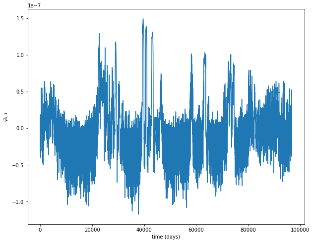
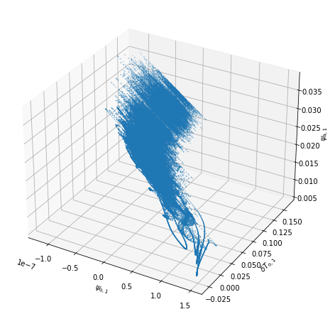
and plot \(\psi_{{\rm a}, 1}\), \(\psi_{{\rm o}, 1}\) and \(\delta T_{{\rm o}, 1}\)
varx = 20
vary = 30
varz = 0

fig = plt.figure(figsize=(10, 8))
axi = fig.gca(projection='3d')

axi.scatter(traj[varx], traj[vary], traj[varz], s=0.2);

axi.set_xlabel('$'+model_parameters.latex_var_string[varx]+'$')
axi.set_ylabel('$'+model_parameters.latex_var_string[vary]+'$')
axi.set_zlabel('$'+model_parameters.latex_var_string[varz]+'$');
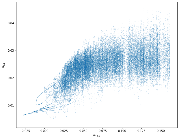
varx = 30
vary = 10
plt.figure(figsize=(10, 8))

plt.plot(traj[varx], traj[vary], marker='o', ms=0.1, ls='')

plt.xlabel('$'+model_parameters.latex_var_string[varx]+'$')
plt.ylabel('$'+model_parameters.latex_var_string[vary]+'$');
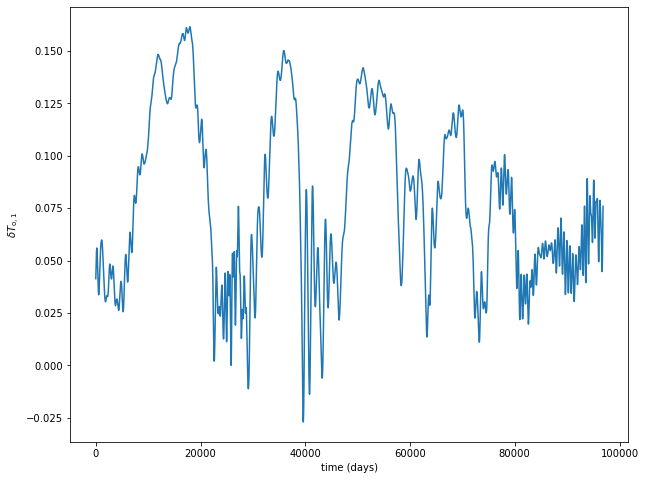
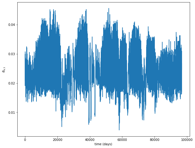
var = 30
plt.figure(figsize=(10, 8))

plt.plot(model_parameters.dimensional_time*time, traj[var])

plt.xlabel('time (days)')
plt.ylabel('$'+model_parameters.latex_var_string[var]+'$');
var = 10
plt.figure(figsize=(10, 8))

plt.plot(model_parameters.dimensional_time*time, traj[var])

plt.xlabel('time (days)')
plt.ylabel('$'+model_parameters.latex_var_string[var]+'$');
var = 20
plt.figure(figsize=(10, 8))

plt.plot(model_parameters.dimensional_time*time, traj[var])

plt.xlabel('time (days)')
plt.ylabel('$'+model_parameters.latex_var_string[var]+'$');