Code Description

In general (see the exception below), the ordinary differential equations (ODEs) of the qgs model are at most bilinear in their variables \(\eta_i\) (\(1\leq i\leq\) ndim). This system of ODEs can therefore be expressed as the sum of a constant, a matrix multiplication, and a tensor contraction:

\[\frac{\mathrm{d}\eta_i}{\mathrm{d}t} = c_i + \sum_{j=1}^{\mathrm{ndim}} m_{i,j} \; \eta_j + \sum_{j,k=1}^{\mathrm{ndim}} t_{i,j,k} \eta_j \eta_k\]

This expression can be further simplified by adding a dummy variable that is identically equal to one: \(\eta_0\equiv 1\). This extra variable allows one to merge \(c_i\), \(m_{i,j}\), and \(t_{i,j,k}\) into the tensor \(\mathcal{T}_{i,j,k}\), in which the linear terms are represented by \(\mathcal{T}_{i,j,0}\) and the constant term by \(\mathcal{T}_{i,0,0}\):

\[\frac{\text{d}\eta_i}{\text{d}t} = \sum_{j,k=0}^{\mathrm{ndim}} \mathcal{T}_{i,j,k} \, \eta_j \, \eta_k\]

The tensor \(\mathcal{T}\) is computed and stored in the QgsTensor. Recasting the system of ordinary differential equations for \(\eta_i\) in the form of a tensor contraction has certain advantages. Indeed, the symmetry of the tensor contraction allows for a unique representation of \(\mathcal{T}_{i,j,k}\), if it is taken to be upper triangular in the last two indices (\(\mathcal{T}_{i,j,k} \equiv 0\) if \(j > k\)). Since \(\mathcal{T}_{i,j,k}\) is known to be sparse, it is stored using the coordinate list representation, i.e. a list of tuples \((i,j,k,\mathcal{T}_{i,j,k})\) defined by the class sparse.COO. This representation renders the computation of the tendencies \(\text{d}\eta_i/\text{d}t\) computationally very efficient as well as conveniently parallelizable.

The form of the ODEs allows also to easily compute the Jacobian matrix of the system. Indeed, denoting the right-hand side of the equations as \(\text{d}\eta_i/\text{d}t = f_i\), the expression reduces to

\[\begin{split}J_{i,j} = \frac{\text{d}f_i}{\text{d}\eta_j}& = \frac{\text{d}}{\text{d}\eta_j } (\sum_{k,l=0}^\mathrm{ndim} \mathcal{T}_{i,k,l} \; \eta_k \; \eta_l ) \\ & = \sum_{k=0}^{\mathrm{ndim}} \left ( \mathcal{T}_{i,k,j} + \mathcal{T}_{i,j,k} \right) \eta_k\end{split}\]

The differential form of the tangent linear model (TL) for a small perturbation \(\boldsymbol{\delta\eta}^\text{TL}\) of a trajectory \(\boldsymbol{\eta}^{\ast}\) is then simply [Kal03]

\[\begin{split}\frac{\text{d}\delta\eta_i^\text{TL}}{\text{d}t} &= \sum_{j=1}^\mathrm{ndim} J^{\ast}_{i,j} \; \delta\eta_j^\text{TL} \\ &= \sum_{j=1}^\mathrm{ndim} \sum_{k=0}^\mathrm{ndim} \left ( \mathcal{T}_{i,k,j} + \mathcal{T}_{i,j,k} \right) \eta^{\ast}_k \; \delta\eta_j^\text{TL}\end{split}\]

Special case with the quartic temperature scheme

In case the quartic temperature scheme is activated, as detailed in the section Dynamical temperatures and quartic temperature tendencies model version, then the above system of ODEs becomes

\[\frac{\text{d}\eta_i}{\text{d}t} = \sum_{j,k,l,m=0}^{\mathrm{ndim}} \mathcal{T}_{i,j,k,l,m} \, \eta_j \, \eta_k \, \eta_l \, \eta_m\]

The Jacobian matrix becomes

\[\begin{split}J_{i,j} = \frac{\text{d}f_i}{\text{d}\eta_j}& = \frac{\text{d}}{\text{d}\eta_j } (\sum_{k,l,m,n=0}^\mathrm{ndim} \mathcal{T}_{i,k,l,m,n} \; \eta_k \; \eta_l \; \eta_m \; \eta_n ) \\ & = \sum_{k,m,n=0}^{\mathrm{ndim}} \left( \mathcal{T}_{i,j,k,m,n} + \mathcal{T}_{i,k,j,m,n} + \mathcal{T}_{i,k,m,j,n} + \mathcal{T}_{i,k,m,n,j}\right) \eta_k \; \eta_m \; \eta_n\end{split}\]

and the tangent linear model can be shown to be provided by the following equation:

\[\begin{split}\frac{\text{d}\delta\eta_i^\text{TL}}{\text{d}t} &= \sum_{j=1}^\mathrm{ndim} J^{\ast}_{i,j} \; \delta\eta_j^\text{TL} \\ &= \sum_{j=1}^\mathrm{ndim} \sum_{k,m,n=0}^\mathrm{ndim} \left( \mathcal{T}_{i,j,k,m,n} + \mathcal{T}_{i,k,j,m,n} + \mathcal{T}_{i,k,m,j,n} + \mathcal{T}_{i,k,m,n,j}\right) \eta^\ast_k \; \eta^\ast_m \; \eta^\ast_n\; \delta\eta_j^\text{TL}\end{split}\]

Computational flow

The computational flow is as follows:

1. The parameters are specified by instantiating a QgParams .

2. The inner products are computed and stored in AtmosphericInnerProducts and OceanicInnerProducts objects.

3. The tensor of the tendencies terms are computed in a QgsTensor object.

4. The functions create_tendencies create Numba optimized functions that return the tendencies and the Jacobian matrix.

5. These functions are passed to the numerical integrator in the module integrator .

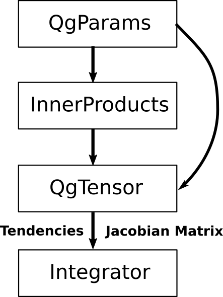
Sketch of the computational flow.

Additional technical information

• qgs is optimized to run ensembles of initial conditions on multiple cores, using Numba jit-compilation and multiprocessing workers.

• qgs has a tangent linear model optimized to run ensembles of initial conditions as well, with a broadcast integration of the tangent model thanks to Numpy.

References

Kal03

E. Kalnay. Atmospheric modeling, data assimilation, and predictability. Cambridge university press, 2003.