Example of the tangent linear and adjoint models usage
Preamble
This notebook shows how to use and integrate the tangent linear and ajoint models.
Reinhold and Pierrehumbert 1982 model version
This notebook use the model version with a simple 2-layer channel QG atmosphere truncated at wavenumber 2 on a beta-plane with a simple orography (a montain and a valley).
More detail can be found in the articles:
Reinhold, B. B., & Pierrehumbert, R. T. (1982). Dynamics of weather regimes: Quasi-stationary waves and blocking. Monthly Weather Review, 110 (9), 1105-1145. doi:10.1175/1520-0493(1982)110%3C1105:DOWRQS%3E2.0.CO;2
Cehelsky, P., & Tung, K. K. (1987). Theories of multiple equilibria and weather regimes—A critical reexamination. Part II: Baroclinic two-layer models. Journal of the atmospheric sciences, 44 (21), 3282-3303. doi:10.1175/1520-0469(1987)044%3C3282%3ATOMEAW%3E2.0.CO%3B2
Modules import
Loading of some modules…
import numpy as np
import matplotlib.pyplot as plt
from mpl_toolkits.mplot3d import Axes3D
Initializing the random number generator (for reproducibility). – Disable if needed.
np.random.seed(210217)
Importing the model’s modules
from qgs.params.params import QgParams
from qgs.integrators.integrator import RungeKuttaIntegrator, RungeKuttaTglsIntegrator
from qgs.functions.tendencies import create_tendencies
from qgs.plotting.util import std_plot
Systems definition
General parameters
# Time parameters
dt = 0.1
# Saving the model state n steps
write_steps = 5

number_of_trajectories = 1
number_of_perturbed_trajectories = 10
Setting some model parameters
# Model parameters instantiation with some non-default specs
model_parameters = QgParams({'phi0_npi': np.deg2rad(50.)/np.pi, 'hd':0.3})
# Mode truncation at the wavenumber 2 in both x and y spatial coordinate
model_parameters.set_atmospheric_channel_fourier_modes(2, 2)

# Changing (increasing) the orography depth and the meridional temperature gradient
model_parameters.ground_params.set_orography(0.4, 1)
model_parameters.atemperature_params.set_thetas(0.2, 0)
# Printing the model's parameters
model_parameters.print_params()
Qgs v1.0.0 parameters summary
=============================

General Parameters:
'dynamic_T': False,
'T4': False,
'time_unit': days,
'rr': 287.058  [J][kg^-1][K^-1]  (gas constant of dry air),
'sb': 5.67e-08  [J][m^-2][s^-1][K^-4]  (Stefan-Boltzmann constant),

Scale Parameters:
'scale': 5000000.0  [m]  (characteristic space scale (L*pi)),
'f0': 0.0001032  [s^-1]  (Coriolis parameter at the middle of the domain),
'n': 1.3    (aspect ratio (n = 2 L_y / L_x)),
'rra': 6370000.0  [m]  (earth radius),
'phi0_npi': 0.2777777777777778    (latitude expressed in fraction of pi),
'deltap': 50000.0  [Pa]  (pressure difference between the two atmospheric layers),

Atmospheric Parameters:
'kd': 0.1  [nondim]  (atmosphere bottom friction coefficient),
'kdp': 0.01  [nondim]  (atmosphere internal friction coefficient),
'sigma': 0.2  [nondim]  (static stability of the atmosphere),

Atmospheric Temperature Parameters:
'hd': 0.3  [nondim]  (Newtonian cooling coefficient),
'thetas[1]': 0.2    (spectral components 1 of the temperature profile),
'thetas[2]': 0.0    (spectral component 2 of the temperature profile),
'thetas[3]': 0.0    (spectral component 3 of the temperature profile),
'thetas[4]': 0.0    (spectral component 4 of the temperature profile),
'thetas[5]': 0.0    (spectral component 5 of the temperature profile),
'thetas[6]': 0.0    (spectral component 6 of the temperature profile),
'thetas[7]': 0.0    (spectral component 7 of the temperature profile),
'thetas[8]': 0.0    (spectral component 8 of the temperature profile),
'thetas[9]': 0.0    (spectral component 9 of the temperature profile),
'thetas[10]': 0.0    (spectral component 10 of the temperature profile),

Ground Parameters:
'hk[1]': 0.0    (spectral component 1 of the orography),
'hk[2]': 0.4    (spectral components 2 of the orography),
'hk[3]': 0.0    (spectral component 3 of the orography),
'hk[4]': 0.0    (spectral component 4 of the orography),
'hk[5]': 0.0    (spectral component 5 of the orography),
'hk[6]': 0.0    (spectral component 6 of the orography),
'hk[7]': 0.0    (spectral component 7 of the orography),
'hk[8]': 0.0    (spectral component 8 of the orography),
'hk[9]': 0.0    (spectral component 9 of the orography),
'hk[10]': 0.0    (spectral component 10 of the orography),
'orographic_basis': atmospheric,
Creating the tendencies function
f, Df = create_tendencies(model_parameters)
Time integration to obtain an initial condition
Defining an integrator
integrator = RungeKuttaIntegrator()
integrator.set_func(f)
Start on a random initial condition and integrate over a transient time to obtain an initial condition on the attractors
ic = np.random.rand(model_parameters.ndim)*0.1
integrator.integrate(0., 200000., dt, ic=ic, write_steps=0)
time, ic = integrator.get_trajectories()
Initial condition sensitivity analysis example
Instantiating a tangent linear integrator with the model tendencies and Jacobian matrix
tgls_integrator = RungeKuttaTglsIntegrator()
tgls_integrator.set_func(f, Df)
Integrating with slightly perturbed initial conditions
tangent_ic = 0.0005*np.random.randn(number_of_perturbed_trajectories, model_parameters.ndim)
tgls_integrator.integrate(0., 180., dt=dt, write_steps=write_steps, ic=ic, tg_ic=tangent_ic)
Obtaining the perturbed trajectories
tt, traj, delta = tgls_integrator.get_trajectories()
pert_traj = traj + delta
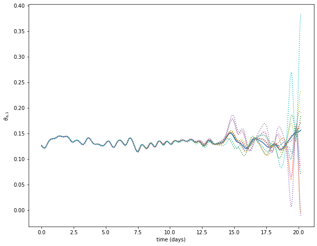
Trajectories plot
var = 10
plt.figure(figsize=(10, 8))

plt.plot(model_parameters.dimensional_time*tt, traj[var])
plt.plot(model_parameters.dimensional_time*tt, pert_traj[:,var].T, ls=':')

ax = plt.gca()

plt.xlabel('time (days)')
plt.ylabel('$'+model_parameters.latex_var_string[var]+'$');
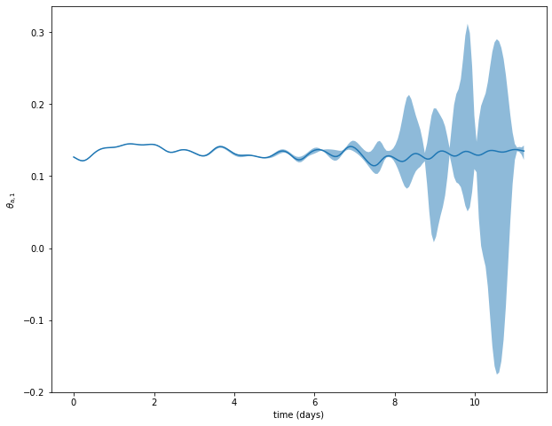
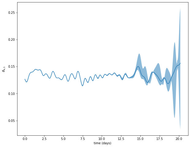
Mean and standard deviation
var = 10
plt.figure(figsize=(10, 8))

plt.plot(model_parameters.dimensional_time*tt, traj[var])

ax = plt.gca()
std_plot(model_parameters.dimensional_time*tt, np.mean(pert_traj[:,var], axis=0), np.sqrt(np.var(pert_traj[:, var], axis=0)), ax=ax, alpha=0.5)

plt.xlabel('time (days)')
plt.ylabel('$'+model_parameters.latex_var_string[var]+'$');
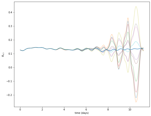
Integrating the adjoint model
Integrating the adjoint model is quite simple and can be done with the same code, simply changing one of the integrator’s parameter:
tgls_integrator.integrate(0., 100., dt=dt, write_steps=write_steps, ic=ic, tg_ic=tangent_ic, adjoint=True)
Obtaining the perturbed trajectories
tt, traj, delta = tgls_integrator.get_trajectories()
pert_traj = traj + delta
Trajectories plot
var = 10
plt.figure(figsize=(10, 8))

plt.plot(model_parameters.dimensional_time*tt, traj[var])
plt.plot(model_parameters.dimensional_time*tt, pert_traj[:,var].T, ls=':')

ax = plt.gca()

plt.xlabel('time (days)')
plt.ylabel('$'+model_parameters.latex_var_string[var]+'$');
Mean and standard deviation
var = 10
plt.figure(figsize=(10, 8))

plt.plot(model_parameters.dimensional_time*tt, traj[var])

ax = plt.gca()
std_plot(model_parameters.dimensional_time*tt, np.mean(pert_traj[:,var], axis=0), np.sqrt(np.var(pert_traj[:, var], axis=0)), ax=ax, alpha=0.5)

plt.xlabel('time (days)')
plt.ylabel('$'+model_parameters.latex_var_string[var]+'$');