Recovering the result of Reinhold and Pierrehumbert (1982)
In this example, we will recover the attractor shown in
Reinhold, B. B., & Pierrehumbert, R. T. (1982). Dynamics of weather regimes: Quasi-stationary waves and blocking. Monthly Weather Review, 110 (9), 1105-1145. doi:10.1175/1520-0493(1982)110%3C1105:DOWRQS%3E2.0.CO;2
obtained with a 2-layer channel QG atmosphere truncated at wavenumber 2 on a beta-plane and a simple orography (a mountain and a valley).
Modules import
Loading of some modules…
import numpy as np
import matplotlib.pyplot as plt
from mpl_toolkits.mplot3d import Axes3D
Initializing the random number generator (for reproducibility). – Disable if needed.
np.random.seed(210217)
Importing the model’s modules
from qgs.params.params import QgParams
from qgs.integrators.integrator import RungeKuttaIntegrator, RungeKuttaTglsIntegrator
from qgs.functions.tendencies import create_tendencies
from qgs.plotting.util import std_plot
and diagnostics
from qgs.diagnostics.streamfunctions import MiddleAtmosphericStreamfunctionDiagnostic
from qgs.diagnostics.variables import VariablesDiagnostic
from qgs.diagnostics.multi import MultiDiagnostic
Systems definition
General parameters
# Time parameters
dt = 0.1
# Saving the model state n steps
write_steps = 5

number_of_trajectories = 1
number_of_perturbed_trajectories = 10
Setting some model parameters
# Model parameters instantiation with some non-default specs
model_parameters = QgParams({'phi0_npi': np.deg2rad(50.)/np.pi, 'hd':0.045})
# Mode truncation at the wavenumber 2 in both x and y spatial coordinate
model_parameters.set_atmospheric_channel_fourier_modes(2, 2)

# Setting the orography depth and the meridional temperature gradient
model_parameters.ground_params.set_orography(0.2, 1)
model_parameters.atemperature_params.set_thetas(0.1, 0)
# Printing the model's parameters
model_parameters.print_params()
Qgs v1.0.0 parameters summary
=============================

General Parameters:
'dynamic_T': False,
'T4': False,
'time_unit': days,
'rr': 287.058  [J][kg^-1][K^-1]  (gas constant of dry air),
'sb': 5.67e-08  [J][m^-2][s^-1][K^-4]  (Stefan-Boltzmann constant),

Scale Parameters:
'scale': 5000000.0  [m]  (characteristic space scale (L*pi)),
'f0': 0.0001032  [s^-1]  (Coriolis parameter at the middle of the domain),
'n': 1.3    (aspect ratio (n = 2 L_y / L_x)),
'rra': 6370000.0  [m]  (earth radius),
'phi0_npi': 0.2777777777777778    (latitude expressed in fraction of pi),
'deltap': 50000.0  [Pa]  (pressure difference between the two atmospheric layers),

Atmospheric Parameters:
'kd': 0.1  [nondim]  (atmosphere bottom friction coefficient),
'kdp': 0.01  [nondim]  (atmosphere internal friction coefficient),
'sigma': 0.2  [nondim]  (static stability of the atmosphere),

Atmospheric Temperature Parameters:
'hd': 0.045  [nondim]  (Newtonian cooling coefficient),
'thetas[1]': 0.1    (spectral components 1 of the temperature profile),
'thetas[2]': 0.0    (spectral component 2 of the temperature profile),
'thetas[3]': 0.0    (spectral component 3 of the temperature profile),
'thetas[4]': 0.0    (spectral component 4 of the temperature profile),
'thetas[5]': 0.0    (spectral component 5 of the temperature profile),
'thetas[6]': 0.0    (spectral component 6 of the temperature profile),
'thetas[7]': 0.0    (spectral component 7 of the temperature profile),
'thetas[8]': 0.0    (spectral component 8 of the temperature profile),
'thetas[9]': 0.0    (spectral component 9 of the temperature profile),
'thetas[10]': 0.0    (spectral component 10 of the temperature profile),

Ground Parameters:
'hk[1]': 0.0    (spectral component 1 of the orography),
'hk[2]': 0.2    (spectral components 2 of the orography),
'hk[3]': 0.0    (spectral component 3 of the orography),
'hk[4]': 0.0    (spectral component 4 of the orography),
'hk[5]': 0.0    (spectral component 5 of the orography),
'hk[6]': 0.0    (spectral component 6 of the orography),
'hk[7]': 0.0    (spectral component 7 of the orography),
'hk[8]': 0.0    (spectral component 8 of the orography),
'hk[9]': 0.0    (spectral component 9 of the orography),
'hk[10]': 0.0    (spectral component 10 of the orography),
'orographic_basis': atmospheric,
Creating the tendencies function
f, Df = create_tendencies(model_parameters)
Time integration and plotting a section of the attractor
Defining an integrator
integrator = RungeKuttaIntegrator()
integrator.set_func(f)
Start on a random initial condition and integrate over a transient time to obtain an initial condition on the attractors
ic = np.random.rand(model_parameters.ndim)*0.1
integrator.integrate(0., 200000., dt, ic=ic, write_steps=0)
time, ic = integrator.get_trajectories()
Now integrate to obtain a trajectory on the attractor
integrator.integrate(0., 100000., dt, ic=ic, write_steps=write_steps)
time, traj = integrator.get_trajectories()
and plot \(\psi_{{\rm a}, 2}\) as a function of \(\psi_{{\rm a}, 3}\)
varx = 2
vary = 1
plt.figure(figsize=(10, 8))

plt.plot(traj[varx], traj[vary], marker='o', ms=0.07, ls='')

plt.xlabel('$'+model_parameters.latex_var_string[varx]+'$')
plt.ylabel('$'+model_parameters.latex_var_string[vary]+'$');
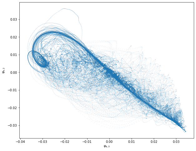
to recover the figure 3 of the Reinhold and Pierrehumbert article mentioned above.
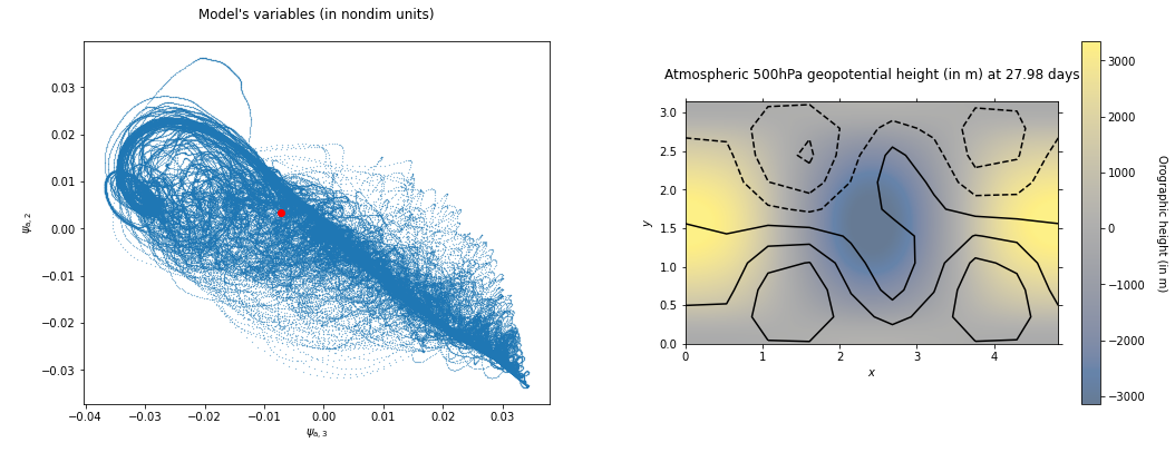
Showing the resulting fields
One can use objects called Diagnostic to plot movies of the model
fields. Here we show how to use them and plot the simultaneous time
evolution of the variables \(\psi_{{\rm a}, 2}\) and
\(\psi_{{\rm a}, 3}\), and the geopotential height field at 500 hPa
over the orographic height.
Creating the diagnostics:
For the 500hPa geopotential height:
psi = MiddleAtmosphericStreamfunctionDiagnostic(model_parameters, geopotential=True)
For the nondimensional variables \(\psi_{{\rm a}, 2}\) and \(\psi_{{\rm a}, 3}\):
variable_nondim = VariablesDiagnostic([2, 1], model_parameters, False)
# setting also the background
background = VariablesDiagnostic([2, 1], model_parameters, False)
background.set_data(time, traj)
Creating a multi diagnostic with both:
m = MultiDiagnostic(1,2)
m.add_diagnostic(variable_nondim, diagnostic_kwargs={'show_time': False, 'background': background}, plot_kwargs={'ms': 0.2})
m.add_diagnostic(psi, diagnostic_kwargs={'style': 'contour', 'contour_labels': False}, plot_kwargs={'colors': 'k'})
m.set_data(time[:501], traj[:501])
and create the movie:
m.movie(figsize=(15,6), anim_kwargs={'interval': 100, 'frames': 500})