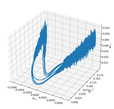
Recovering the result of De Cruz, Demaeyer and Vannitsem (2016)
In this example, we recover the attractor shown in
De Cruz, L., Demaeyer, J. and Vannitsem, S. (2016). The Modular Arbitrary-Order Ocean-Atmosphere Model: MAOOAM v1.0, Geosci. Model Dev., 9, 2793-2808. doi:10.5194/gmd-9-2793-2016
obtained with a 2-layer channel QG atmosphere truncated at wavenumber 2 coupled, both by friction and heat exchange, to a shallow water ocean with 8 modes.
Modules import
Loading of some modules…
import numpy as np
import matplotlib.pyplot as plt
from mpl_toolkits.mplot3d import Axes3D
Initializing the random number generator (for reproducibility). – Disable if needed.
np.random.seed(21217)
Importing the model’s modules
from qgs.params.params import QgParams
from qgs.integrators.integrator import RungeKuttaIntegrator
from qgs.functions.tendencies import create_tendencies
and diagnostics
from qgs.diagnostics.streamfunctions import MiddleAtmosphericStreamfunctionDiagnostic, OceanicLayerStreamfunctionDiagnostic
from qgs.diagnostics.temperatures import MiddleAtmosphericTemperatureDiagnostic, OceanicLayerTemperatureDiagnostic
from qgs.diagnostics.variables import VariablesDiagnostic, GeopotentialHeightDifferenceDiagnostic
from qgs.diagnostics.multi import MultiDiagnostic
Systems definition
General parameters
# Time parameters
dt = 0.1
# Saving the model state n steps
write_steps = 10

number_of_trajectories = 1
Setting some model parameters
# Model parameters instantiation with some non-default specs
model_parameters = QgParams()

# Mode truncation at the wavenumber 2 in both x and y spatial
# coordinates for the atmosphere
model_parameters.set_atmospheric_channel_fourier_modes(2, 2)
# Mode truncation at the wavenumber 2 in the x and at the
# wavenumber 4 in the y spatial coordinates for the ocean
model_parameters.set_oceanic_basin_fourier_modes(2, 4)
# Setting MAOOAM parameters according to the publication linked above
model_parameters.set_params({'kd': 0.0290, 'kdp': 0.0290, 'n': 1.5, 'r': 1.e-7,
                             'h': 136.5, 'd': 1.1e-7})
model_parameters.atemperature_params.set_params({'eps': 0.7, 'T0': 289.3,
                                                 'hlambda': 15.06})
model_parameters.gotemperature_params.set_params({'gamma': 5.6e8, 'T0': 301.46})
Setting the short-wave radiation component as in the publication above: \(C_{\text{a},1}\) and \(C_{\text{o},1}\)
model_parameters.atemperature_params.set_insolation(103.3333, 0)
model_parameters.gotemperature_params.set_insolation(310, 0)
Printing the model’s parameters
model_parameters.print_params()
Qgs v1.0.0 parameters summary
=============================

General Parameters:
'dynamic_T': False,
'T4': False,
'time_unit': days,
'rr': 287.058  [J][kg^-1][K^-1]  (gas constant of dry air),
'sb': 5.67e-08  [J][m^-2][s^-1][K^-4]  (Stefan-Boltzmann constant),

Scale Parameters:
'scale': 5000000.0  [m]  (characteristic space scale (L*pi)),
'f0': 0.0001032  [s^-1]  (Coriolis parameter at the middle of the domain),
'n': 1.5    (aspect ratio (n = 2 L_y / L_x)),
'rra': 6370000.0  [m]  (earth radius),
'phi0_npi': 0.25    (latitude expressed in fraction of pi),
'deltap': 50000.0  [Pa]  (pressure difference between the two atmospheric layers),

Atmospheric Parameters:
'kd': 0.029  [nondim]  (atmosphere bottom friction coefficient),
'kdp': 0.029  [nondim]  (atmosphere internal friction coefficient),
'sigma': 0.2  [nondim]  (static stability of the atmosphere),

Atmospheric Temperature Parameters:
'gamma': 10000000.0  [J][m^-2][K^-1]  (specific heat capacity of the atmosphere),
'C[1]': 103.3333  [W][m^-2]  (spectral component 1 of the short-wave radiation of the atmosphere),
'C[2]': 0.0  [W][m^-2]  (spectral component 2 of the short-wave radiation of the atmosphere),
'C[3]': 0.0  [W][m^-2]  (spectral component 3 of the short-wave radiation of the atmosphere),
'C[4]': 0.0  [W][m^-2]  (spectral component 4 of the short-wave radiation of the atmosphere),
'C[5]': 0.0  [W][m^-2]  (spectral component 5 of the short-wave radiation of the atmosphere),
'C[6]': 0.0  [W][m^-2]  (spectral component 6 of the short-wave radiation of the atmosphere),
'C[7]': 0.0  [W][m^-2]  (spectral component 7 of the short-wave radiation of the atmosphere),
'C[8]': 0.0  [W][m^-2]  (spectral component 8 of the short-wave radiation of the atmosphere),
'C[9]': 0.0  [W][m^-2]  (spectral component 9 of the short-wave radiation of the atmosphere),
'C[10]': 0.0  [W][m^-2]  (spectral component 10 of the short-wave radiation of the atmosphere),
'eps': 0.7    (emissivity coefficient for the grey-body atmosphere),
'T0': 289.3  [K]  (stationary solution for the 0-th order atmospheric temperature),
'sc': 1.0    (ratio of surface to atmosphere temperature),
'hlambda': 15.06  [W][m^-2][K^-1]  (sensible+turbulent heat exchange between ocean and atmosphere),

Oceanic Parameters:
'gp': 0.031  [m][s^-2]  (reduced gravity),
'r': 1e-07  [s^-1]  (frictional coefficient at the bottom of the ocean),
'h': 136.5  [m]  (depth of the water layer of the ocean),
'd': 1.1e-07  [s^-1]  (strength of the ocean-atmosphere mechanical coupling),

Oceanic Temperature Parameters:
'gamma': 560000000.0  [J][m^-2][K^-1]  (specific heat capacity of the ocean),
'C[1]': 310.0  [W][m^-2]  (spectral component 0 of the short-wave radiation of the ocean),
'C[2]': 0.0  [W][m^-2]  (spectral component 1 of the short-wave radiation of the ocean),
'C[3]': 0.0  [W][m^-2]  (spectral component 2 of the short-wave radiation of the ocean),
'C[4]': 0.0  [W][m^-2]  (spectral component 3 of the short-wave radiation of the ocean),
'C[5]': 0.0  [W][m^-2]  (spectral component 4 of the short-wave radiation of the ocean),
'C[6]': 0.0  [W][m^-2]  (spectral component 5 of the short-wave radiation of the ocean),
'C[7]': 0.0  [W][m^-2]  (spectral component 6 of the short-wave radiation of the ocean),
'C[8]': 0.0  [W][m^-2]  (spectral component 7 of the short-wave radiation of the ocean),
'C[9]': 0.0  [W][m^-2]  (spectral component 8 of the short-wave radiation of the ocean),
'C[10]': 0.0  [W][m^-2]  (spectral component 9 of the short-wave radiation of the ocean),
'T0': 301.46  [K]  (stationary solution for the 0-th order oceanic temperature),
Creating the tendencies function
f, Df = create_tendencies(model_parameters)
Time integration and plotting a section of the attractor
Defining an integrator
integrator = RungeKuttaIntegrator()
integrator.set_func(f)
Start on a random initial condition and integrate over a transient time to obtain an initial condition on the attractors (may take several minutes)
## Might take several minutes, depending on your cpu computational power.
ic = np.random.rand(model_parameters.ndim)*0.01
integrator.integrate(0., 10000000., dt, ic=ic, write_steps=0)
time, ic = integrator.get_trajectories()
Now integrate to obtain a trajectory on the attractor
integrator.integrate(0., 1000000., dt, ic=ic, write_steps=write_steps)
time, traj = integrator.get_trajectories()
and plot \(\psi_{{\rm a}, 1}\), \(\psi_{{\rm o}, 2}\) and \(\delta T_{{\rm o}, 2}\)
fig = plt.figure(figsize=(10, 8))
axi = fig.gca(projection='3d')

axi.scatter(traj[21], traj[29], traj[0], s=0.2);

axi.set_xlabel('$'+model_parameters.latex_var_string[21]+'$')
axi.set_ylabel('$'+model_parameters.latex_var_string[29]+'$')
axi.set_zlabel('$'+model_parameters.latex_var_string[0]+'$');
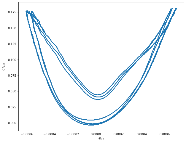
varx = 21
vary = 29
plt.figure(figsize=(10, 8))

plt.plot(traj[varx], traj[vary], marker='o', ms=0.1, ls='')

plt.xlabel('$'+model_parameters.latex_var_string[varx]+'$')
plt.ylabel('$'+model_parameters.latex_var_string[vary]+'$');
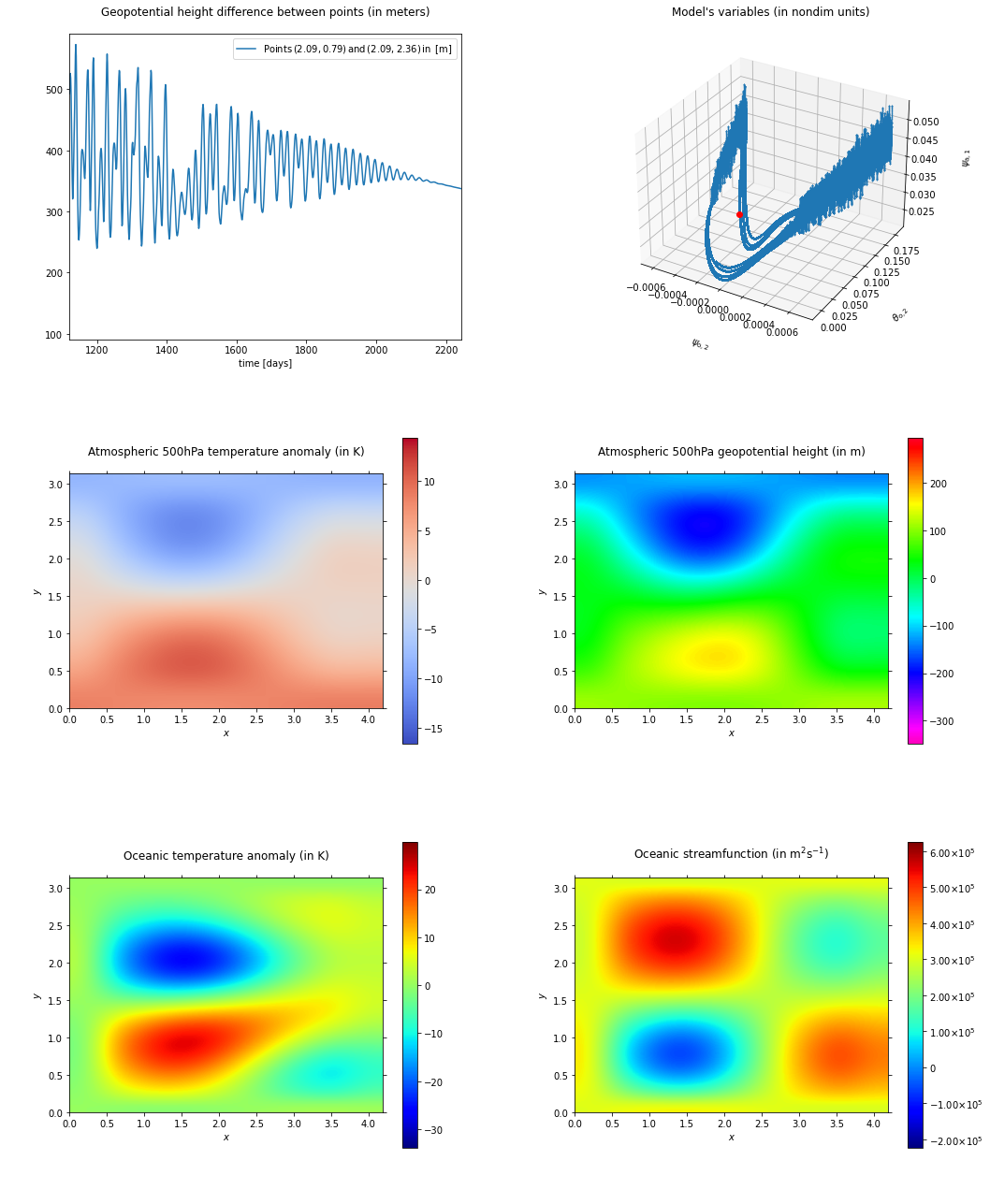
Showing the resulting fields
One can use objects called Diagnostic to plot movies of the model
fields. Here we show how to use them and plot the simultaneous time
evolution of the variables \(\psi_{{\rm a}, 1}\),
\(\psi_{{\rm o}, 2}\) and \(\delta T_{{\rm o}, 2}\), with the
corresponding atmospheric and oceanic streamfunctions and temperature at
500 hPa.
First, we create the diagnostics:
For the 500hPa geopotential height:
psi_a = MiddleAtmosphericStreamfunctionDiagnostic(model_parameters, geopotential=True)
For the 500hPa atmospheric temperature:
theta_a = MiddleAtmosphericTemperatureDiagnostic(model_parameters)
For the ocean streamfunction:
psi_o = OceanicLayerStreamfunctionDiagnostic(model_parameters)
For the ocean temperature:
theta_o = OceanicLayerTemperatureDiagnostic(model_parameters)
For the nondimensional variables \(\psi_{{\rm a}, 1}\), \(\psi_{{\rm o}, 2}\) and \(\delta T_{{\rm o}, 2}\):
variable_nondim = VariablesDiagnostic([21, 29, 0], model_parameters, False)
For the geopotential height difference between North and South:
geopot_dim = GeopotentialHeightDifferenceDiagnostic([[[np.pi/model_parameters.scale_params.n, np.pi/4], [np.pi/model_parameters.scale_params.n, 3*np.pi/4]]],
                                                    model_parameters, True)
# setting also the background
background = VariablesDiagnostic([21, 29, 0], model_parameters, False)
background.set_data(time, traj)
and we select a subset of the data to plot:
stride = 10
sel_time = time[10000:10000+5200*stride:stride]
sel_traj = traj[:, 10000:10000+5200*stride:stride]
We then create a multi diagnostic with all the diagnostics:
m = MultiDiagnostic(3,2)
m.add_diagnostic(geopot_dim, diagnostic_kwargs={'style':'moving-timeserie'})
m.add_diagnostic(variable_nondim, diagnostic_kwargs={'show_time':False, 'background': background, 'style':'3Dscatter'}, plot_kwargs={'ms': 0.2})
m.add_diagnostic(theta_a, diagnostic_kwargs={'show_time':False})
m.add_diagnostic(psi_a, diagnostic_kwargs={'show_time':False})
m.add_diagnostic(theta_o, diagnostic_kwargs={'show_time':False})
m.add_diagnostic(psi_o, diagnostic_kwargs={'show_time':False})

m.set_data(sel_time, sel_traj)
and create the movie:
m.movie(figsize=(15,18), anim_kwargs={'interval': 100, 'frames':1000})