Example of DiffEqPy usage
Preamble
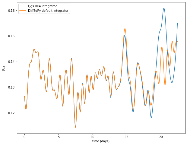
This notebook shows how to use the DiffEqPy package to integrate the qgs model and compare with the qgs Runge-Kutta integrator.
Reinhold and Pierrehumbert 1982 model version
This notebook use the model version with a simple 2-layer channel QG atmosphere truncated at wavenumber 2 on a beta-plane with a simple orography (a montain and a valley).
More detail can be found in the articles:
Reinhold, B. B., & Pierrehumbert, R. T. (1982). Dynamics of weather regimes: Quasi-stationary waves and blocking. Monthly Weather Review, 110 (9), 1105-1145. doi:10.1175/1520-0493(1982)110%3C1105:DOWRQS%3E2.0.CO;2
Cehelsky, P., & Tung, K. K. (1987). Theories of multiple equilibria and weather regimes—A critical reexamination. Part II: Baroclinic two-layer models. Journal of the atmospheric sciences, 44 (21), 3282-3303. doi:10.1175/1520-0469(1987)044%3C3282%3ATOMEAW%3E2.0.CO%3B2
Modules import
Loading of some modules…
import numpy as np
import matplotlib.pyplot as plt
from mpl_toolkits.mplot3d import Axes3D
Initializing the random number generator (for reproducibility). – Disable if needed.
np.random.seed(210217)
Importing the model’s modules
from qgs.params.params import QgParams
from qgs.integrators.integrator import RungeKuttaIntegrator
from qgs.functions.tendencies import create_tendencies
from qgs.plotting.util import std_plot
Importing Julia DifferentialEquations.jl package
from julia.api import Julia
jl = Julia(compiled_modules=False)
from diffeqpy import de
Importing also Numba
from numba import jit
Systems definition
General parameters
# Time parameters
dt = 0.1
# Saving the model state n steps
write_steps = 5

number_of_trajectories = 1
number_of_perturbed_trajectories = 10
Setting some model parameters
# Model parameters instantiation with some non-default specs
model_parameters = QgParams({'phi0_npi': np.deg2rad(50.)/np.pi, 'hd':0.3})
# Mode truncation at the wavenumber 2 in both x and y spatial coordinate
model_parameters.set_atmospheric_channel_fourier_modes(2, 2)

# Changing (increasing) the orography depth and the meridional temperature gradient
model_parameters.ground_params.set_orography(0.4, 1)
model_parameters.atemperature_params.set_thetas(0.2, 0)
# Printing the model's parameters
model_parameters.print_params()
Qgs v1.0.0 parameters summary
=============================

General Parameters:
'dynamic_T': False,
'T4': False,
'time_unit': days,
'rr': 287.058  [J][kg^-1][K^-1]  (gas constant of dry air),
'sb': 5.67e-08  [J][m^-2][s^-1][K^-4]  (Stefan-Boltzmann constant),

Scale Parameters:
'scale': 5000000.0  [m]  (characteristic space scale (L*pi)),
'f0': 0.0001032  [s^-1]  (Coriolis parameter at the middle of the domain),
'n': 1.3    (aspect ratio (n = 2 L_y / L_x)),
'rra': 6370000.0  [m]  (earth radius),
'phi0_npi': 0.2777777777777778    (latitude expressed in fraction of pi),
'deltap': 50000.0  [Pa]  (pressure difference between the two atmospheric layers),

Atmospheric Parameters:
'kd': 0.1  [nondim]  (atmosphere bottom friction coefficient),
'kdp': 0.01  [nondim]  (atmosphere internal friction coefficient),
'sigma': 0.2  [nondim]  (static stability of the atmosphere),

Atmospheric Temperature Parameters:
'hd': 0.3  [nondim]  (Newtonian cooling coefficient),
'thetas[1]': 0.2    (spectral components 1 of the temperature profile),
'thetas[2]': 0.0    (spectral component 2 of the temperature profile),
'thetas[3]': 0.0    (spectral component 3 of the temperature profile),
'thetas[4]': 0.0    (spectral component 4 of the temperature profile),
'thetas[5]': 0.0    (spectral component 5 of the temperature profile),
'thetas[6]': 0.0    (spectral component 6 of the temperature profile),
'thetas[7]': 0.0    (spectral component 7 of the temperature profile),
'thetas[8]': 0.0    (spectral component 8 of the temperature profile),
'thetas[9]': 0.0    (spectral component 9 of the temperature profile),
'thetas[10]': 0.0    (spectral component 10 of the temperature profile),

Ground Parameters:
'hk[1]': 0.0    (spectral component 1 of the orography),
'hk[2]': 0.4    (spectral components 2 of the orography),
'hk[3]': 0.0    (spectral component 3 of the orography),
'hk[4]': 0.0    (spectral component 4 of the orography),
'hk[5]': 0.0    (spectral component 5 of the orography),
'hk[6]': 0.0    (spectral component 6 of the orography),
'hk[7]': 0.0    (spectral component 7 of the orography),
'hk[8]': 0.0    (spectral component 8 of the orography),
'hk[9]': 0.0    (spectral component 9 of the orography),
'hk[10]': 0.0    (spectral component 10 of the orography),
'orographic_basis': atmospheric,
Creating the tendencies function
f, Df = create_tendencies(model_parameters)
Time integration
Defining an integrator
integrator = RungeKuttaIntegrator()
integrator.set_func(f)
Start on a random initial condition and integrate over a transient time to obtain an initial condition on the attractors
ic = np.random.rand(model_parameters.ndim)*0.1
integrator.integrate(0., 200000., dt, ic=ic, write_steps=0)
time, ic = integrator.get_trajectories()
Now integrate to obtain with the qgs RK4 integrator
integrator.integrate(0., 200., dt, ic=ic, write_steps=write_steps)
time, traj = integrator.get_trajectories()
And also with the DifferentialEquations ODE Solver
# defining a function with a DifferentialEquations.jl compatible header

@jit
def f_jl(x,p,t):
    u = f(t,x)
    return u
# Defining the problem and integrating
prob = de.ODEProblem(f_jl, ic, (0., 200.))
sol = de.solve(prob, saveat=write_steps * dt)
Plotting the result
var = 10
jtraj = np.array(sol.u).T
plt.figure(figsize=(10, 8))

plt.plot(model_parameters.dimensional_time*time, traj[var], label="Qgs RK4 integrator")
plt.plot(model_parameters.dimensional_time*time, jtraj[var], label="DiffEqPy default integrator")

plt.legend()
plt.xlabel('time (days)')
plt.ylabel('$'+model_parameters.latex_var_string[var]+'$');