Model with an orography and a temperature profile

An orography and a mean potential temperature profile can be added to the system. The resulting model is described in detail in [CS80] and [RP82].

Friction with the ground

The atmosphere is coupled to the orography through mechanical coupling (friction).

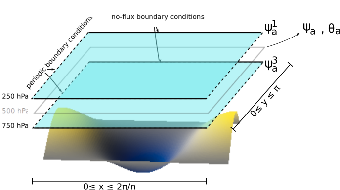
Sketch of the atmospheric model layers with a simple orography. The domain (\(\beta\)-plane) nondimensional zonal and meridional coordinates are labeled as the \(x\) and \(y\) variables.

It transforms the equations in Atmospheric component into

\[\begin{split}\frac{\partial}{\partial t} \left(\nabla^2 \psi^1_{\rm a}\right)+ J(\psi^1_{\rm a}, \nabla^2 \psi^1_{\rm a})+ \beta \frac{\partial \psi^1_{\rm a}}{\partial x} & = -k'_d \nabla^2 (\psi^1_{\rm a}-\psi^3_{\rm a})+ \frac{f_0}{\Delta p} \omega \nonumber \\ \frac{\partial}{\partial t} \left( \nabla^2 \psi^3_{\rm a} \right) + J(\psi^3_{\rm a}, \nabla^2 \psi^3_{\rm a}) + J(\psi^3_{\rm a}, f_0 \, h/H_{\rm a}) + \beta \frac{\partial \psi^3_{\rm a}}{\partial x} & = +k'_d \nabla^2 (\psi^1_{\rm a}-\psi^3_{\rm a}) - k_d \nabla^2 \psi^3_{\rm a} - \frac{f_0}{\Delta p} \omega \nonumber \\\end{split}\]

where \(H_{\rm a}\) is the characteristic depth of each fluid layer and the parameter \(k_d\) (kd) quantifies the friction between the atmosphere and the surface. \(h\) is the topographic height field.

Mid-layer equations and the thermal wind relation

The equations governing the time evolution of the mean and shear streamfunctions \(\psi_{\rm a} = (\psi^1_{\rm a} + \psi^3_{\rm a})/2\) and \(\theta_{\rm a} = (\psi^1_{\rm a} - \psi^3_{\rm a})/2\) is given by

\[\begin{split}&\frac{\partial}{\partial t} \left(\nabla^2 \psi_{\rm a}\right) + J(\psi_{\rm a}, \nabla^2 \psi_{\rm a}) + J(\theta_{\rm a}, \nabla^2 \theta_{\rm a}) + \frac{1}{2} J(\psi_{\rm a} - \theta_{\rm a}, f_0 \, h/H_{\rm a}) + \beta \frac{\partial \psi_{\rm a}}{\partial x} = - \frac{k_d}{2} \nabla^2 (\psi_{\rm a} - \theta_{\rm a}) \\ &\frac{\partial}{\partial t} \left( \nabla^2 \theta_{\rm a} \right) + J(\psi_{\rm a}, \nabla^2 \theta_{\rm a}) + J(\theta_{\rm a}, \nabla^2 \psi_{\rm a}) - \frac{1}{2} J(\psi_{\rm a} - \theta_{\rm a}, f_0 \, h/H_{\rm a}) + \beta \frac{\partial \theta_{\rm a}}{\partial x} \nonumber \\ & \qquad \qquad \qquad \qquad \qquad \qquad = - 2 \, k'_d \nabla^2 \theta_{\rm a} + \frac{k_d}{2} \nabla^2 (\psi_{\rm a} - \theta_{\rm a}) + \frac{f_0}{\Delta p} \omega.\end{split}\]

\(\psi_{\rm a}\) and \(\theta_{\rm a}\) are often referred to as the barotropic and baroclinic streamfunctions, respectively. On the other hand, the thermodynamic equation governing the mean potential temperature \(T_{\rm a} = (T^1_{\rm a} + T^3_{\rm a})/2\), where \(T^1_{\rm a}\) and \(T^3_{\rm a}\) are the mean potential temperature in respectively the upper and lower layer, is given by [Val06]

\[\frac{\partial}{\partial t} T_{\rm a} + J(\psi_{\rm a}, T_{\rm a}) = \frac{\sigma \, \Delta p}{R} \,\omega + h_d \, (T^\ast - T_{\rm a})\]

where \(h_d\) (hd) is the Newtonian cooling coefficient indicating the tendency to return to the equilibrium temperature profile \(T^\ast\). \(\sigma\) (sigma) is the static stability of the atmosphere, taken to be constant.

The hydrostatic relation in pressure coordinates is \((\partial \Phi/\partial p) = -1/\rho_\text{a}\) with the geopotential height \(\Phi = f_0\;\psi_\text{a}\) and \(\rho_\text{a}\) the dry air density. The ideal gas relation \(p=\rho_\text{a} R T_\text{a}\) and the vertical discretization of the hydrostatic relation at 500 hPa allows to write the spatially dependent atmospheric temperature anomaly \(\delta T_\text{a} = 2f_0\;\theta_\text{a} /R\) where \(R\) (rr) is the ideal gas constant. Therefore, upon nondimensionalization, both fields are identified with each other: \(2 \theta_{\rm a} \equiv T_{\rm a}\) and \(2 \theta^\star \equiv T^\star\), and the equations above fully describe the system.

The mean streamfunction \(\psi_{\rm a}\) and temperature \(\theta_{\rm a}\) can be considered to be the value of these fields at the 500 hPa level.

Projecting the equations on a set of basis functions

The present model solves the equations above by projecting them onto a set of basis functions, to obtain a system of ordinary differential equations (ODE). This procedure is sometimes called a Galerkin expansion. This basis being finite, the resolution of the model is automatically truncated at the characteristic length of the highest-resolution function of the basis.

Both fields are defined in a zonally periodic channel with no-flux boundary conditions in the meridional direction (\(\partial \cdot /\partial x \equiv 0\) at the meridional boundaries).

The fields are projected on Fourier modes respecting these boundary conditions:

\[\begin{split}&F^A_{P} (x, y) = \sqrt{2}\, \cos(P y), \\ &F^K_{M,P} (x, y) = 2\cos(M nx)\, \sin(P y), \\ &F^L_{H,P} (x, y) = 2\sin(H nx)\, \sin(P y)\end{split}\]

with integer values of \(M\), \(H\), \(P\). \(x\) and \(y\) are the horizontal adimensionalized coordinates, rescaled by dividing the dimensional coordinates by the characteristic length \(L\) (L). The model’s domain is then defined by \((0 \leq x \leq \frac{2\pi}{n}, 0 \leq y \leq \pi)\), with \(n\) (n) the aspect ratio between its meridional and zonal extents \(L_y\) (L_y) and \(L_x\) (L_x).

To easily manipulate these functions and the coefficients of the fields expansion, we number the basis functions along increasing values of \(M= H\) and then \(P\). It allows to write the set as \(\left\{ F_i(x,y); 1 \leq i \leq n_\text{a}\right\}\) where \(n_{\mathrm{a}}\) (nmod [0]) is the number of modes of the spectral expansion.

For example, with \(M=H=1\) and \(P \in \{1,2\}\), one obtains the spectral truncation used by [CS80]. The model derived in [RP82] extended this set by two blocks of two functions each, and the resulting set can be specified as \(M,H \in \{1,2\}\); \(P \in \{1,2\}\). The corresponding set of basis functions is

\[\begin{split}F_1(x,y) & = & \sqrt{2}\, \cos(y), \nonumber \\ F_2(x,y) & = & 2\, \cos(n x)\, \sin(y), \nonumber \\ F_3(x,y) & = & 2\, \sin(n x)\, \sin(y), \nonumber \\ F_4(x,y) & = & \sqrt{2}\, \cos(2y), \nonumber \\ F_5(x,y) & = & 2 \cos(n x) \sin(2y), \nonumber \\ F_6(x,y) & = & 2 \sin(n x) \sin(2y), \nonumber \\ & \vdots & \nonumber\end{split}\]

such that

\[\nabla^2 F_i(x,y) = -a^2_i F_i(x,y)\]

with eigenvalues \(a_i^2 = P_i^2 + n^2 \, M_i^2\) or \(a_i^2 = P_i^2 + n^2 \, H_i^2\). These Fourier modes are orthonormal with respect to the inner product

\[\frac{n}{2\pi^2}\int_0^\pi\int_0^{2\pi/n} F_i(x,y)\, F_j(x,y)\, \mathrm{d} x \, \mathrm{d} y = \delta_{ij}\]

where \(\delta_{ij}\) is the Kronecker delta.

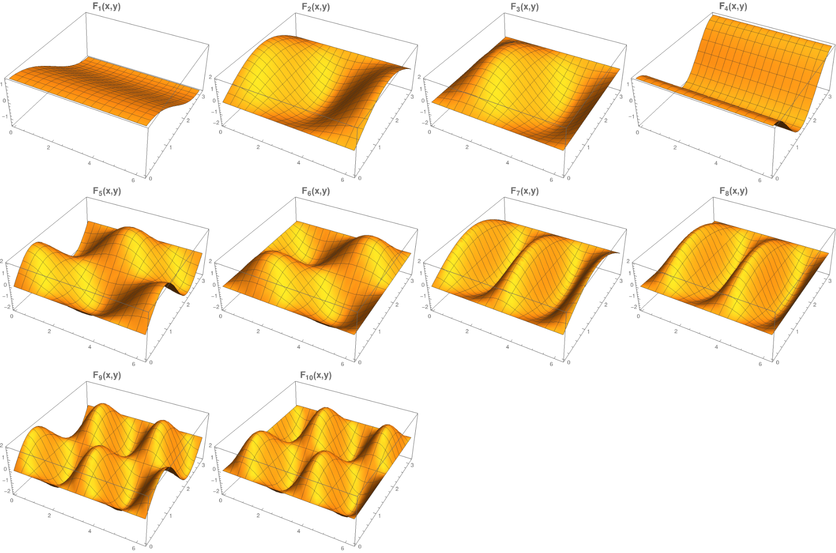
The first 10 basis functions \(F_i\) evaluated on the nondimensional domain of the model.

The model’s fields can be decomposed as follows:

\[\begin{split}\psi_{\rm a}(x,y) & = & \sum_{i=1}^{n_{\mathrm{a}}} \, \psi_{{\rm a},i} \, F_i(x,y) \\ \theta_{\rm a}(x,y) & = & \sum_{i=1}^{n_{\mathrm{a}}} \, \theta_{{\rm a},i} \, F_i(x,y) .\end{split}\]

The radiative equilibrium temperature field \(\theta^\star(x,y)\), the topographic height field \(h(x,y)\) and the vertical velocity \(\omega(x,y)\) also have to be decomposed into the eigenfunctions of the Laplacian:

\[\begin{split}\theta^\star(x,y) & = & \sum_{i=1}^{n_{\mathrm{a}}} \, \theta^\star_i \, F_i(x,y) \\ h(x,y) & = & \sum_{i=1}^{n_{\mathrm{a}}} \, h_i \, F_i(x,y) \\ \omega(x,y) & = & \sum_{i=1}^{n_{\mathrm{a}}} \, \omega_i \, F_i(x,y) .\end{split}\]

These fields can be specified in the model by setting the (non-dimensional) vectors hk and thetas. Note that \(h\) is scaled by the characteristic height \(H_{\rm a}\) of each layer, and \(\theta^\star\) is scaled by \(A f_0^2 L^2\) (see section below).

Ordinary differential equations

The fields, parameters and variables are non-dimensionalized by dividing time by \(f_0^{-1}\) (f0), distance by the characteristic length scale \(L\) (L), pressure by the difference \(\Delta p\) (deltap), temperature by \(A f_0^2 L^2\), and streamfunction by \(L^2 f_0\). As stated above, a result of this non-dimensionalization is that the field \(\theta_{\rm a}\) is identified with \(T_{\rm a}\): \(\theta_{\rm a} \equiv T_{\rm a}\).

The ordinary differential equations of the truncated model are:

\[\begin{split}\dot\psi_{{\rm a},i} & = & - a_{i,i}^{-1} \sum_{j,m = 1}^{n_{\mathrm{a}}} b_{i, j, m} \left(\psi_{{\rm a},j}\, \psi_{{\rm a},m} + \theta_{{\rm a},j}\, \theta_{{\rm a},m}\right) - \frac{a_{i,i}^{-1}}{2} \sum_{j,m = 1}^{n_{\mathrm{a}}} g_{i, j, m} \, h_m \left(\psi_{{\rm a},j}-\theta_{{\rm a},j}\right) \nonumber \\ & & \qquad \qquad \qquad \qquad - \beta\, a_{i,i}^{-1} \, \sum_{j=1}^{n_{\mathrm{a}}} \, c_{i, j} \, \psi_{{\rm a},j} - \frac{k_d}{2} \left(\psi_{{\rm a},i} - \theta_{{\rm a},i}\right) \\ \dot\theta_{\rm{a},i} & = & - a_{i,i}^{-1} \sum_{j,m = 1}^{n_{\mathrm{a}}} b_{i, j, m} \left(\psi_{{\rm a},j}\, \theta_{{\rm a},m} + \theta_{{\rm a},j}\, \psi_{{\rm a},m}\right) + \frac{a_{i,i}^{-1}}{2} \sum_{j,m = 1}^{n_{\mathrm{a}}} g_{i, j, m} \, h_m \left(\psi_{{\rm a},j}-\theta_{{\rm a},j}\right) \nonumber \\ & & \qquad \qquad \qquad \qquad - \beta\, a_{i,i}^{-1} \, \sum_{j=1}^{n_{\mathrm{a}}} \, c_{i, j} \, \theta_{{\rm a},j} + \frac{k_d}{2} \left(\psi_{{\rm a},i} - \theta_{{\rm a},i}\right) -2 \, k'_d \, \theta_{{\rm a},i} + a_{i,i}^{-1} \, \omega_i \\ \dot\theta_{\rm{a},i} & = & - \sum_{j,m = 1}^{n_{\mathrm{a}}} g_{i, j, m} \, \psi_{{\rm a},j}\, \theta_{{\rm a},m} + \frac{\sigma}{2} \, \omega_i + h_d \, \left(\theta^\ast_i - \theta_{{\rm a},i}\right)\end{split}\]

where the parameters values have been replaced by their non-dimensional ones. The coefficients \(a_{i,j}\), \(g_{i, j, m}\), \(b_{i, j, m}\) and \(c_{i, j}\) are the inner products of the Fourier modes \(F_i\):

\[\begin{split}a_{i,j} & = & \frac{n}{2\pi^2}\int_0^\pi\int_0^{2\pi/n} F_i(x,y)\, \nabla^2 F_j(x,y)\, \mathrm{d} x \, \mathrm{d} y = - \delta_{ij} \, a_i^2 \\ g_{i, j, m} & = & \frac{n}{2\pi^2}\int_0^\pi\int_0^{2\pi/n} F_i(x,y)\, J\left(F_j(x,y), F_m(x,y)\right) \, \mathrm{d} x \, \mathrm{d} y \\ b_{i, j, m} & = & \frac{n}{2\pi^2}\int_0^\pi\int_0^{2\pi/n} F_i(x,y)\, J\left(F_j(x,y), \nabla^2 F_m(x,y)\right) \, \mathrm{d} x \, \mathrm{d} y \\ c_{i, j} & = & \frac{n}{2\pi^2}\int_0^\pi\int_0^{2\pi/n} F_i(x,y)\, \frac{\partial}{\partial x} F_j(x,y) \, \mathrm{d} x \, \mathrm{d} y\end{split}\]

These inner products are computed according to formulas found in [CT87] and stored in an object derived from the AtmosphericInnerProducts class.

The vertical velocity \(\omega_i\) can be eliminated, leading to the final equations

\[\begin{split}\dot\psi_{{\rm a},i} & = & - a_{i,i}^{-1} \sum_{j,m = 1}^{n_{\mathrm{a}}} b_{i, j, m} \left(\psi_{{\rm a},j}\, \psi_{{\rm a},m} + \theta_{{\rm a},j}\, \theta_{{\rm a},m}\right) - \frac{a_{i,i}^{-1}}{2} \sum_{j,m = 1}^{n_{\mathrm{a}}} g_{i, j, m} \, h_m \left(\psi_{{\rm a},j}-\theta_{{\rm a},j}\right) \nonumber \\ & & \qquad \qquad \qquad \qquad - \beta\, a_{i,i}^{-1} \, \sum_{j=1}^{n_{\mathrm{a}}} \, c_{i, j} \, \psi_{{\rm a},j} - \frac{k_d}{2} \left(\psi_{{\rm a},i} - \theta_{{\rm a},i}\right) \\ \dot\theta_{{\rm a},i} & = & \frac{\sigma/2}{a_{i,i} \,\sigma/2 - 1} \left\{ - \sum_{j,m = 1}^{n_{\mathrm{a}}} b_{i, j, m} \left(\psi_{{\rm a},j}\, \theta_{{\rm a},m} + \theta_{{\rm a},j}\, \psi_{{\rm a},m}\right) + \frac{1}{2} \sum_{j,m = 1}^{n_{\mathrm{a}}} g_{i, j, m} \, h_m \left(\psi_{{\rm a},j}-\theta_{{\rm a},j}\right) \right. \nonumber \\ & & \quad - \left. \beta\, \, \sum_{j=1}^{n_{\mathrm{a}}} \, c_{i, j} \, \theta_{{\rm a},j} + \frac{k_d}{2} \, a_{i,i} \left(\psi_{{\rm a},i} - \theta_{{\rm a},i}\right) -2 \, k'_d \, a_{i,i} \, \theta_{{\rm a},i} \right\} \nonumber \\ & & + \frac{1}{a_{i,i} \,\sigma/2 - 1} \left\{ \sum_{j,m = 1}^{n_{\mathrm{a}}} g_{i, j, m} \, \psi_{{\rm a},j}\, \theta_{{\rm a},m} - h_d \, \left(\theta^\ast_i - \theta_{{\rm a},i}\right)\right\}\end{split}\]

that are implemented in with a tensorial contraction:

\[\frac{\text{d}\eta_{{\rm{a},i}}}{\text{d}t} = \sum_{j, k=0}^{2 n_\mathrm{a}} \mathcal{T}_{i,j,k} \; \eta_{{\rm a},j} \; \eta_{{\rm a},k}\]

with \(\boldsymbol{\eta_{\mathrm{a}}} = (\psi_{{\rm a},1}, \ldots, \psi_{{\rm a},n_\mathrm{a}}, \theta_{{\rm a},1}, \ldots, \theta_{{\rm a},n_\mathrm{a}})\), as described in the Code Description. The tensor \(\mathcal{T}\) is computed and stored in the QgsTensor.

Example

An example about how to setup the model to use this model version is shown in Recovering the result of Reinhold and Pierrehumbert (1982).

References

CT87

P. Cehelsky and K. K. Tung. Theories of multiple equilibria and weather regimes - A critical reexamination. Part II: Baroclinic two-layer models. Journal of the Atmospheric Sciences, 44(21):3282–3303, 1987. URL: https://doi.org/10.1175/1520-0469(1987)044%3C3282:TOMEAW%3E2.0.CO;2.

CS80(1,2)

J. Charney and D. Straus. Form-drag instability, multiple equilibria and propagating planetary waves in baroclinic, orographically forced, planetary wave systems. Journal of the Atmospheric Sciences, 37(6):1157–1176, 1980. URL: https://doi.org/10.1175/1520-0469(1980)037%3C1157:FDIMEA%3E2.0.CO;2.

RP82(1,2)

B. Reinhold and R. Pierrehumbert. Dynamics of weather regimes: quasi-stationary waves and blocking. Monthly Weather Review, 110:1105–1145, 1982. URL: https://doi.org/10.1175/1520-0493(1982)110%3C1105:DOWRQS%3E2.0.CO;2.

Val06

G. K. Vallis. Atmospheric and oceanic fluid dynamics: fundamentals and large-scale circulation. Cambridge University Press, 2006.