Manual setting of the basis
In this example, we show how to setup a user-defined basis. It is done here for the ocean, but the approach is the same for the other components. We will project the ocean equations on four modes proposed in
S. Pierini. Low-frequency variability, coherence resonance, and phase selection in a low-order model of the wind-driven ocean circulation. Journal of Physical Oceanography, 41(9):1585–1604, 2011. doi:10.1175/JPO-D-10-05018.1.
S. Vannitsem and L. De Cruz. A 24-variable low-order coupled ocean–atmosphere model: OA-QG-WS v2. Geoscientific Model Development, 7(2):649–662, 2014. doi:10.5194/gmd-7-649-2014.
These four modes are given by
\(\tilde\phi_1(x,y)=2 \, e^{−\alpha x} \sin(n x/2) \sin(y)\)
\(\tilde\phi_2(x,y)=2 \, e^{−\alpha x} \sin(n x) \sin(y)\)
\(\tilde\phi_3(x,y)=2 \, e^{−\alpha x} \sin(n x/2) \sin(2y)\)
\(\tilde\phi_4(x,y)=2 \, e^{−\alpha x} \sin(n x) \sin(2y)\)
This ocean is then connected to a channel atmosphere using a symbolic basis of functions.
Modules import
Loading of some modules…
import sys, os, warnings
sys.path.extend([os.path.abspath('../')])
import numpy as np
import matplotlib.pyplot as plt
from numba import njit
Initializing the random number generator (for reproducibility). – Disable if needed.
np.random.seed(210217)
Importing the model’s modules
from qgs.params.params import QgParams
from qgs.basis.base import SymbolicBasis
from qgs.inner_products.definition import StandardSymbolicInnerProductDefinition
from qgs.inner_products.symbolic import AtmosphericSymbolicInnerProducts, OceanicSymbolicInnerProducts
from qgs.tensors.qgtensor import QgsTensor
from qgs.functions.sparse_mul import sparse_mul3
from qgs.integrators.integrator import RungeKuttaIntegrator
and diagnostics
from qgs.diagnostics.streamfunctions import MiddleAtmosphericStreamfunctionDiagnostic, OceanicLayerStreamfunctionDiagnostic
from qgs.diagnostics.temperatures import MiddleAtmosphericTemperatureDiagnostic, OceanicLayerTemperatureDiagnostic
from qgs.diagnostics.variables import VariablesDiagnostic, GeopotentialHeightDifferenceDiagnostic
from qgs.diagnostics.multi import MultiDiagnostic
and some SymPy functions
from sympy import symbols, sin, exp, pi
Systems definition
General parameters
# Time parameters
dt = 0.1
# Saving the model state n steps
write_steps = 100
number_of_trajectories = 1
Setting some model parameters and setting the atmosphere basis
# Model parameters instantiation with some non-default specs
model_parameters = QgParams({'n': 1.5})
# Mode truncation at the wavenumber 2 in both x and y spatial
# coordinates for the atmosphere
model_parameters.set_atmospheric_channel_fourier_modes(2, 2, mode="symbolic")
Creating the ocean basis
ocean_basis = SymbolicBasis()
x, y = symbols('x y') # x and y coordinates on the model's spatial domain
n, al = symbols('n al', real=True, nonnegative=True) # aspect ratio and alpha coefficients
for i in range(1, 3):
for j in range(1, 3):
ocean_basis.functions.append(2 * exp(- al * x) * sin(j * n * x / 2) * sin(i * y))
Setting the value of the parameter α to a certain value (here α=1). Please note that the α is then an extrinsic parameter of the model that you have to specify through a substitution:
ocean_basis.substitutions.append((al, 1.))
ocean_basis.substitutions.append((n, model_parameters.scale_params.n))
Setting now the ocean basis
model_parameters.set_oceanic_modes(ocean_basis)
Additionally, for these particular ocean basis functions, a special inner product needs to be defined instead of the standard one proposed. We thus set up a new definition for the ocean component as in the publication linked above:
class UserInnerProductDefinition(StandardSymbolicInnerProductDefinition):
def symbolic_inner_product(self, S, G, symbolic_expr=False, integrand=False):
"""Function defining the inner product to be computed symbolically:
:math:`(S, G) = \\frac{n}{2\\pi^2}\\int_0^\\pi\\int_0^{2\\pi/n} e^{2 \\alpha x} \\, S(x,y)\\, G(x,y)\\, \\mathrm{d} x \\, \\mathrm{d} y`.
Parameters
----------
S: Sympy expression
Left-hand side function of the product.
G: Sympy expression
Right-hand side function of the product.
symbolic_expr: bool, optional
If `True`, return the integral as a symbolic expression object. Else, return the integral performed symbolically.
integrand: bool, optional
If `True`, return the integrand of the integral and its integration limits as a list of symbolic expression object. Else, return the integral performed symbolically.
Returns
-------
Sympy expression
The result of the symbolic integration
"""
expr = (n / (2 * pi ** 2)) * exp(2 * al * x) * S * G
if integrand:
return expr, (x, 0, 2 * pi / n), (y, 0, pi)
else:
return self.integrate_over_domain(self.optimizer(expr), symbolic_expr=symbolic_expr)
Finally setting some other model’s parameters:
# Setting MAOOAM parameters according to the publication linked above
model_parameters.set_params({'kd': 0.029, 'kdp': 0.029, 'r': 1.0e-7,
'h': 136.5, 'd': 1.1e-7})
model_parameters.atemperature_params.set_params({'eps': 0.76, 'T0': 289.3,
'hlambda': 15.06})
model_parameters.gotemperature_params.set_params({'gamma': 5.6e8, 'T0': 301.46})
Setting the short-wave radiation component as in the publication above: \(C_{\text{a},1}\) and \(C_{\text{o},1}\)
model_parameters.atemperature_params.set_insolation(103.3333, 0)
model_parameters.gotemperature_params.set_insolation(310, 0)
Printing the model’s parameters
model_parameters.print_params()
Qgs v1.0.0 parameters summary
=============================
General Parameters:
'dynamic_T': False,
'T4': False,
'time_unit': days,
'rr': 287.058 [J][kg^-1][K^-1] (gas constant of dry air),
'sb': 5.67e-08 [J][m^-2][s^-1][K^-4] (Stefan-Boltzmann constant),
Scale Parameters:
'scale': 5000000.0 [m] (characteristic space scale (L*pi)),
'f0': 0.0001032 [s^-1] (Coriolis parameter at the middle of the domain),
'n': 1.5 (aspect ratio (n = 2 L_y / L_x)),
'rra': 6370000.0 [m] (earth radius),
'phi0_npi': 0.25 (latitude expressed in fraction of pi),
'deltap': 50000.0 [Pa] (pressure difference between the two atmospheric layers),
Atmospheric Parameters:
'kd': 0.029 [nondim] (atmosphere bottom friction coefficient),
'kdp': 0.029 [nondim] (atmosphere internal friction coefficient),
'sigma': 0.2 [nondim] (static stability of the atmosphere),
Atmospheric Temperature Parameters:
'gamma': 10000000.0 [J][m^-2][K^-1] (specific heat capacity of the atmosphere),
'C[1]': 103.3333 [W][m^-2] (spectral component 1 of the short-wave radiation of the atmosphere),
'C[2]': 0.0 [W][m^-2] (spectral component 2 of the short-wave radiation of the atmosphere),
'C[3]': 0.0 [W][m^-2] (spectral component 3 of the short-wave radiation of the atmosphere),
'C[4]': 0.0 [W][m^-2] (spectral component 4 of the short-wave radiation of the atmosphere),
'C[5]': 0.0 [W][m^-2] (spectral component 5 of the short-wave radiation of the atmosphere),
'C[6]': 0.0 [W][m^-2] (spectral component 6 of the short-wave radiation of the atmosphere),
'C[7]': 0.0 [W][m^-2] (spectral component 7 of the short-wave radiation of the atmosphere),
'C[8]': 0.0 [W][m^-2] (spectral component 8 of the short-wave radiation of the atmosphere),
'C[9]': 0.0 [W][m^-2] (spectral component 9 of the short-wave radiation of the atmosphere),
'C[10]': 0.0 [W][m^-2] (spectral component 10 of the short-wave radiation of the atmosphere),
'eps': 0.76 (emissivity coefficient for the grey-body atmosphere),
'T0': 289.3 [K] (stationary solution for the 0-th order atmospheric temperature),
'sc': 1.0 (ratio of surface to atmosphere temperature),
'hlambda': 15.06 [W][m^-2][K^-1] (sensible+turbulent heat exchange between ocean and atmosphere),
Oceanic Parameters:
'gp': 0.031 [m][s^-2] (reduced gravity),
'r': 1e-07 [s^-1] (frictional coefficient at the bottom of the ocean),
'h': 136.5 [m] (depth of the water layer of the ocean),
'd': 1.1e-07 [s^-1] (strength of the ocean-atmosphere mechanical coupling),
Oceanic Temperature Parameters:
'gamma': 560000000.0 [J][m^-2][K^-1] (specific heat capacity of the ocean),
'C[1]': 310.0 [W][m^-2] (spectral component 0 of the short-wave radiation of the ocean),
'C[2]': 0.0 [W][m^-2] (spectral component 1 of the short-wave radiation of the ocean),
'C[3]': 0.0 [W][m^-2] (spectral component 2 of the short-wave radiation of the ocean),
'C[4]': 0.0 [W][m^-2] (spectral component 3 of the short-wave radiation of the ocean),
'C[5]': 0.0 [W][m^-2] (spectral component 4 of the short-wave radiation of the ocean),
'C[6]': 0.0 [W][m^-2] (spectral component 5 of the short-wave radiation of the ocean),
'C[7]': 0.0 [W][m^-2] (spectral component 6 of the short-wave radiation of the ocean),
'C[8]': 0.0 [W][m^-2] (spectral component 7 of the short-wave radiation of the ocean),
'C[9]': 0.0 [W][m^-2] (spectral component 8 of the short-wave radiation of the ocean),
'C[10]': 0.0 [W][m^-2] (spectral component 9 of the short-wave radiation of the ocean),
'T0': 301.46 [K] (stationary solution for the 0-th order oceanic temperature),
We now construct the tendencies of the model by first constructing the ocean and atmosphere inner products objects. In addition, a inner product definition instance defined above must be passed to the ocean inner products object:
with warnings.catch_warnings():
warnings.simplefilter("ignore")
ip = UserInnerProductDefinition()
aip = AtmosphericSymbolicInnerProducts(model_parameters)
oip = OceanicSymbolicInnerProducts(model_parameters, inner_product_definition=ip)
and finally we create manually the tendencies function, first by creating the tensor object:
aotensor = QgsTensor(model_parameters, aip, oip)
and then the Python-Numba callable for the model’s tendencies \(\boldsymbol{f}\) :
coo = aotensor.tensor.coords.T
val = aotensor.tensor.data
@njit
def f(t, x):
xx = np.concatenate((np.full((1,), 1.), x))
xr = sparse_mul3(coo, val, xx, xx)
return xr[1:]
Time integration
Defining an integrator
integrator = RungeKuttaIntegrator()
integrator.set_func(f)
Start on a random initial condition and integrate over a transient time to obtain an initial condition on the attractors
## Might take several minutes, depending on your cpu computational power.
ic = np.random.rand(model_parameters.ndim)*0.0001
integrator.integrate(0., 10000000., dt, ic=ic, write_steps=0)
time, ic = integrator.get_trajectories()
Now integrate to obtain a trajectory on the attractor
integrator.integrate(0., 1000000., dt, ic=ic, write_steps=write_steps)
reference_time, reference_traj = integrator.get_trajectories()
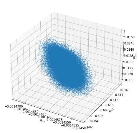
Plotting the result in 3D and 2D
varx = 21
vary = 25
varz = 0
fig = plt.figure(figsize=(10, 8))
axi = fig.add_subplot(111, projection='3d')
axi.scatter(reference_traj[varx], reference_traj[vary], reference_traj[varz], s=0.2);
axi.set_xlabel('$'+model_parameters.latex_var_string[varx]+'$')
axi.set_ylabel('$'+model_parameters.latex_var_string[vary]+'$')
axi.set_zlabel('$'+model_parameters.latex_var_string[varz]+'$');
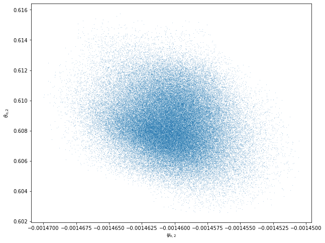
varx = 21
vary = 25
plt.figure(figsize=(10, 8))
plt.plot(reference_traj[varx], reference_traj[vary], marker='o', ms=0.1, ls='')
plt.xlabel('$'+model_parameters.latex_var_string[varx]+'$')
plt.ylabel('$'+model_parameters.latex_var_string[vary]+'$');
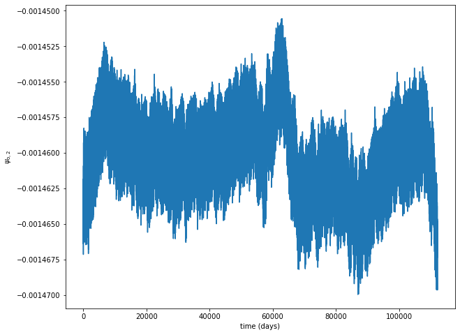
var = 21
plt.figure(figsize=(10, 8))
plt.plot(model_parameters.dimensional_time*reference_time, reference_traj[var])
plt.xlabel('time (days)')
plt.ylabel('$'+model_parameters.latex_var_string[var]+'$');
Showing the resulting fields (animation)
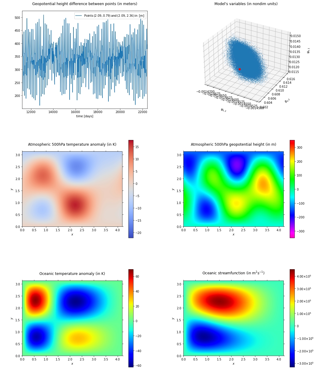
Here, we want to show that the diagnostics adapt to the manually set basis.
One can use objects called Diagnostic to plot movies of the model
fields. Here we show how to use them and plot the simultaneous time
evolution of the variables \(\psi_{{\rm a}, 1}\),
\(\psi_{{\rm o}, 2}\) and \(\delta T_{{\rm o}, 2}\), with the
corresponding atmospheric and oceanic streamfunctions and temperature at
500 hPa.
Creating the diagnostics (for field plots, we must specify the grid step):
For the 500hPa geopotential height:
psi_a = MiddleAtmosphericStreamfunctionDiagnostic(model_parameters, delta_x=0.1, delta_y=0.1, geopotential=True)
For the 500hPa atmospheric temperature:
theta_a = MiddleAtmosphericTemperatureDiagnostic(model_parameters, delta_x=0.1, delta_y=0.1)
For the ocean streamfunction:
psi_o = OceanicLayerStreamfunctionDiagnostic(model_parameters, delta_x=0.1, delta_y=0.1, conserved=False)
For the ocean temperature:
theta_o = OceanicLayerTemperatureDiagnostic(model_parameters, delta_x=0.1, delta_y=0.1)
For the nondimensional variables \(\psi_{{\rm a}, 1}\), \(\psi_{{\rm o}, 2}\) and \(\delta T_{{\rm o}, 2}\):
variable_nondim = VariablesDiagnostic([21, 25, 0], model_parameters, False)
For the geopotential height difference between North and South:
geopot_dim = GeopotentialHeightDifferenceDiagnostic([[[np.pi/model_parameters.scale_params.n, np.pi/4], [np.pi/model_parameters.scale_params.n, 3*np.pi/4]]],
model_parameters, True)
# setting also the background
background = VariablesDiagnostic([21, 25, 0], model_parameters, False)
background.set_data(reference_time, reference_traj)
Selecting a subset of the data to plot:
stride = 10
time = reference_time[10000:10000+5200*stride:stride]
traj = reference_traj[:, 10000:10000+5200*stride:stride]
Creating a multi diagnostic with both:
m = MultiDiagnostic(3,2)
m.add_diagnostic(geopot_dim, diagnostic_kwargs={'style':'moving-timeserie'})
m.add_diagnostic(variable_nondim, diagnostic_kwargs={'show_time':False, 'background': background, 'style':'3Dscatter'}, plot_kwargs={'ms': 0.2})
m.add_diagnostic(theta_a, diagnostic_kwargs={'show_time':False})
m.add_diagnostic(psi_a, diagnostic_kwargs={'show_time':False})
m.add_diagnostic(theta_o, diagnostic_kwargs={'show_time':False})
m.add_diagnostic(psi_o, diagnostic_kwargs={'show_time':False})
m.set_data(time, traj)
and showing finally a movie:
m.movie(figsize=(15,18), anim_kwargs={'interval': 100, 'frames':1000})