Recovering the result of Hamilton et al. (2023)
In this example, we recover results similar to what was shown in
TBD
obtained with a 2-layer channel QG atmosphere truncated at wavenumber 2 coupled, both by friction and heat exchange, to a shallow water ocean with 8 modes, and with a dynamic reference temperature for both components.
Modules import
Loading of some modules…
import numpy as np
import matplotlib.pyplot as plt
from mpl_toolkits.mplot3d import Axes3D
Initializing the random number generator (for reproducibility). – Disable if needed.
np.random.seed(210217)
Importing the model’s modules
from qgs.params.params import QgParams
from qgs.integrators.integrator import RungeKuttaIntegrator
from qgs.functions.tendencies import create_tendencies
and diagnostics
from qgs.diagnostics.streamfunctions import MiddleAtmosphericStreamfunctionDiagnostic, OceanicLayerStreamfunctionDiagnostic
from qgs.diagnostics.temperatures import MiddleAtmosphericTemperatureDiagnostic, OceanicLayerTemperatureDiagnostic
from qgs.diagnostics.variables import VariablesDiagnostic, GeopotentialHeightDifferenceDiagnostic
from qgs.diagnostics.multi import MultiDiagnostic
Systems definition
General parameters
# Time parameters
dt = 0.1
# Saving the model state n steps
write_steps = 100

number_of_trajectories = 1
Setting some model parameters
# Model parameters instantiation with some non-default specs
# Dynamic temperature is activated here with the dynamic_T parameter
# Set also the T4 parameter to true to active the quartic temperature scheme as well
model_parameters = QgParams({'n': 1.5}, dynamic_T=True)
# model_parameters = QgParams({'n': 1.5}, T4=True)

# Modes definition: with dynamic reference temperature, the user has to use the symbolic modes
# Mode truncation at the wavenumber 2 in both x and y spatial
# coordinates for the atmosphere
model_parameters.set_atmospheric_channel_fourier_modes(2, 2, mode="symbolic")
# Mode truncation at the wavenumber 2 in the x and at the
# wavenumber 4 in the y spatial coordinates for the ocean
model_parameters.set_oceanic_basin_fourier_modes(2, 4, mode="symbolic")
# Setting MAOOAM parameters according to the publication linked above
model_parameters.set_params({'kd': 0.0290, 'kdp': 0.0290, 'r': 1.e-7,
                             'h': 136.5, 'd': 1.1e-7})
model_parameters.atemperature_params.set_params({'eps': 0.7, 'hlambda': 15.06})
model_parameters.gotemperature_params.set_params({'gamma': 5.6e8})
Setting the short-wave radiation component as in the publication above: \(C_{\text{a},1}\) and \(C_{\text{o},1}\)
model_parameters.atemperature_params.set_insolation(103., 0)
model_parameters.atemperature_params.set_insolation(103., 1)
model_parameters.gotemperature_params.set_insolation(310., 0)
model_parameters.gotemperature_params.set_insolation(310., 1)
Printing the model’s parameters
model_parameters.print_params()
Qgs v1.0.0 parameters summary
=============================

General Parameters:
'dynamic_T': True,
'T4': False,
'time_unit': days,
'rr': 287.058  [J][kg^-1][K^-1]  (gas constant of dry air),
'sb': 5.67e-08  [J][m^-2][s^-1][K^-4]  (Stefan-Boltzmann constant),

Scale Parameters:
'scale': 5000000.0  [m]  (characteristic space scale (L*pi)),
'f0': 0.0001032  [s^-1]  (Coriolis parameter at the middle of the domain),
'n': 1.5    (aspect ratio (n = 2 L_y / L_x)),
'rra': 6370000.0  [m]  (earth radius),
'phi0_npi': 0.25    (latitude expressed in fraction of pi),
'deltap': 50000.0  [Pa]  (pressure difference between the two atmospheric layers),

Atmospheric Parameters:
'kd': 0.029  [nondim]  (atmosphere bottom friction coefficient),
'kdp': 0.029  [nondim]  (atmosphere internal friction coefficient),
'sigma': 0.2  [nondim]  (static stability of the atmosphere),

Atmospheric Temperature Parameters:
'gamma': 10000000.0  [J][m^-2][K^-1]  (specific heat capacity of the atmosphere),
'C[1]': 103.0  [W][m^-2]  (spectral component 1 of the short-wave radiation of the atmosphere),
'C[2]': 103.0  [W][m^-2]  (spectral component 2 of the short-wave radiation of the atmosphere),
'C[3]': 0.0  [W][m^-2]  (spectral component 3 of the short-wave radiation of the atmosphere),
'C[4]': 0.0  [W][m^-2]  (spectral component 4 of the short-wave radiation of the atmosphere),
'C[5]': 0.0  [W][m^-2]  (spectral component 5 of the short-wave radiation of the atmosphere),
'C[6]': 0.0  [W][m^-2]  (spectral component 6 of the short-wave radiation of the atmosphere),
'C[7]': 0.0  [W][m^-2]  (spectral component 7 of the short-wave radiation of the atmosphere),
'C[8]': 0.0  [W][m^-2]  (spectral component 8 of the short-wave radiation of the atmosphere),
'C[9]': 0.0  [W][m^-2]  (spectral component 9 of the short-wave radiation of the atmosphere),
'C[10]': 0.0  [W][m^-2]  (spectral component 10 of the short-wave radiation of the atmosphere),
'C[11]': 0.0  [W][m^-2]  (spectral component 11 of the short-wave radiation of the atmosphere),
'eps': 0.7    (emissivity coefficient for the grey-body atmosphere),
'sc': 1.0    (ratio of surface to atmosphere temperature),
'hlambda': 15.06  [W][m^-2][K^-1]  (sensible+turbulent heat exchange between ocean and atmosphere),

Oceanic Parameters:
'gp': 0.031  [m][s^-2]  (reduced gravity),
'r': 1e-07  [s^-1]  (frictional coefficient at the bottom of the ocean),
'h': 136.5  [m]  (depth of the water layer of the ocean),
'd': 1.1e-07  [s^-1]  (strength of the ocean-atmosphere mechanical coupling),

Oceanic Temperature Parameters:
'gamma': 560000000.0  [J][m^-2][K^-1]  (specific heat capacity of the ocean),
'C[1]': 310.0  [W][m^-2]  (spectral component 0 of the short-wave radiation of the ocean),
'C[2]': 310.0  [W][m^-2]  (spectral component 1 of the short-wave radiation of the ocean),
'C[3]': 0.0  [W][m^-2]  (spectral component 2 of the short-wave radiation of the ocean),
'C[4]': 0.0  [W][m^-2]  (spectral component 3 of the short-wave radiation of the ocean),
'C[5]': 0.0  [W][m^-2]  (spectral component 4 of the short-wave radiation of the ocean),
'C[6]': 0.0  [W][m^-2]  (spectral component 5 of the short-wave radiation of the ocean),
'C[7]': 0.0  [W][m^-2]  (spectral component 6 of the short-wave radiation of the ocean),
'C[8]': 0.0  [W][m^-2]  (spectral component 7 of the short-wave radiation of the ocean),
'C[9]': 0.0  [W][m^-2]  (spectral component 8 of the short-wave radiation of the ocean),
'C[10]': 0.0  [W][m^-2]  (spectral component 9 of the short-wave radiation of the ocean),
'C[11]': 0.0  [W][m^-2]  (spectral component 10 of the short-wave radiation of the ocean),
Creating the tendencies function
f, Df = create_tendencies(model_parameters)
Time integration and plotting a section of the attractor
Defining an integrator
integrator = RungeKuttaIntegrator()
integrator.set_func(f)
Start on a random initial condition and integrate over a transient time to obtain an initial condition on the attractors (may take several minutes)
## Might take several minutes, depending on your cpu computational power.
ic = np.random.rand(model_parameters.ndim)*0.01
ic[29] = 3.  # Setting reasonable initial reference temperature
ic[10] = 1.5
integrator.integrate(0., 2000000.1, dt, ic=ic, write_steps=0)
time, ic = integrator.get_trajectories()
Now integrate to obtain a trajectory on the attractor
integrator.integrate(0., 3000000., dt, ic=ic, write_steps=write_steps)
reference_time, reference_traj = integrator.get_trajectories()
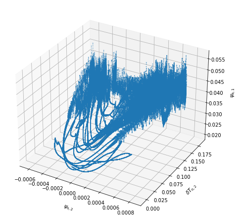
and plot \(\psi_{{\rm a}, 1}\), \(\psi_{{\rm o}, 2}\) and \(\delta T_{{\rm o}, 2}\)
varx = 22
vary = 31
varz = 0

fig = plt.figure(figsize=(10, 8))
axi = fig.add_subplot(111, projection='3d')

axi.scatter(reference_traj[varx], reference_traj[vary], reference_traj[varz], s=0.2);

axi.set_xlabel('$'+model_parameters.latex_var_string[varx]+'$', labelpad=12.)
axi.set_ylabel('$'+model_parameters.latex_var_string[vary]+'$', labelpad=12.)
axi.set_zlabel('$'+model_parameters.latex_var_string[varz]+'$', labelpad=12.);
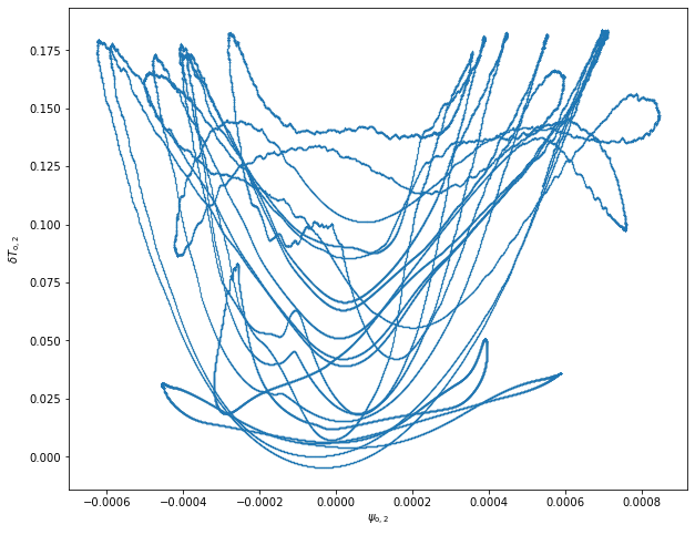
varx = 22
vary = 31
plt.figure(figsize=(10, 8))

plt.plot(reference_traj[varx], reference_traj[vary], marker='o', ms=0.1, ls='')

plt.xlabel('$'+model_parameters.latex_var_string[varx]+'$')
plt.ylabel('$'+model_parameters.latex_var_string[vary]+'$');
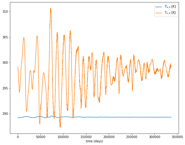
Plot of the atmospheric and oceanic reference temperatures \(T_{{\rm a}, 0}\) and \(T_{{\rm o}, 0}\)
var = 10
plt.figure(figsize=(10, 8))

plt.plot(model_parameters.dimensional_time*reference_time, 2* model_parameters.temperature_scaling * reference_traj[var], label='$'+model_parameters.latex_var_string[var]+'$ [K]')
plt.plot(model_parameters.dimensional_time*reference_time, model_parameters.temperature_scaling * reference_traj[29], label='$'+model_parameters.latex_var_string[29]+'$ [K]')


plt.xlabel('time (days)')
#plt.ylabel();
plt.legend();
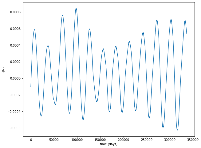
Plot of the low-frequency variability in \(\psi_{{\rm o}, 2}\)
var = 22
plt.figure(figsize=(10, 8))

plt.plot(model_parameters.dimensional_time*reference_time, reference_traj[var])


plt.xlabel('time (days)')
plt.ylabel('$'+model_parameters.latex_var_string[var]+'$');