User guide
This guide explains how the qgs framework can be used and configured to obtain the various model version.
1. Rationale behind qgs
The purpose of qgs is to provide a Python callable representing the model’s tendencies to the user, e.g. to provide a function \(\boldsymbol{f}\) (and also its Jacobian matrix) that can be integrated over time:
to obtain the model’s trajectory. This callable can of course also be used to perform any other kind of model analysis.
This guide provides:
The different ways to configure qgs in order to obtain the function \(\boldsymbol{f}\) are explained in the section 2. Configuration of qgs.
Some specific ways to configure qgs detailed in the section 3. Using user-defined symbolic basis.
Examples of usages of the model’s tendencies function \(\boldsymbol{f}\) are given in the section 5. Using qgs (once configured).
2. Configuration of qgs
The computational flow to compute the function \(\boldsymbol{f}\) of the model’s tendencies \(\dot{\boldsymbol{x}} = \boldsymbol{f}(t, \boldsymbol{x})\) is explained in Computational flow and sketched below:
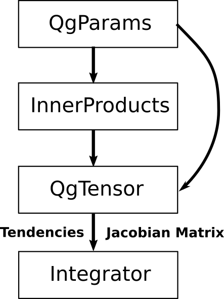
Sketch of the computational flow.
This flow can be implemented step by step by the user, or can be automatically performed by the functions create_tendencies().
This function takes a QgParams parameters object and return the function \(\boldsymbol{f}\) and its Jacobian matrix.
Optionally, it can also return the byproducts of the tendencies generation process, i.e. the objects containing the inner products
between the model’s spatial modes and the tensors of the model’s tendencies terms.
This section of the user guide explains how to configure the QgParams object to obtain the desired model version and
model’s parameters.
2.1 Two different computational methods and three different geophysical components
Two different methods are available to configure qgs, related to two different methods of computing the inner products between its spatial basis functions:
Symbolic: It is the main way to specify the basis. The user can specify an arbitrary basis of functions on which the model’s partial differential equations will be projected. Depending on the dimension of the model version and on the computing power available, it might take a while to initialize.
Analytic: The old method to specify the model version, in which the basis of functions are composed only of Fourier modes described in Coupled ocean-atmosphere model (MAOOAM) and is thus limited in term of modelling capacity. It is nevertheless the fastest way since it relies on analytic formulas derived in [USER-DCDV16] to compute the basis functions.
There are also three different geophysical components presently available in qgs:
Atmosphere: This component is mandatory and provides a two-layers quasi-geostrophic atmosphere. See Atmospheric component for more details.
Ocean: This component provides a shallow-water active oceanic layer. See Oceanic component for more details.
Ground: This component provides a simple model for the ground (orography + heat exchange). It is present by default if only the atmospheric component is defined, but then with only the orography being activated (no heat exchange).
The components needed by the user and their parameters have to be defined by instantiating a QgParams object.
How to create this object, initialize these components and set the parameters of the model is the subject of the next sections.
2.2 Initializing qgs
The model initialization first step requires the creation of a QgParams object:
from qgs.params.params import QgParams
model_parameters = QgParams()
This object contains basically all the information needed by qgs to construct the inner products and the tendencies tensor of the model, which are in turn needed to produces finally the model’s function \(\boldsymbol{f}\).
The different components required by the user need then to be specified, by providing information about the basis of functions used to project the partial differential equations of qgs. As said before, two methods are available:
2.2.1 The symbolic method
With this method, the user has to provide directly the basis of functions of each component. These functions have to be symbolic function expressions, and should be provided using Sympy.
This has to be done using a SymbolicBasis object, which is basically a list of Sympy functions.
The user can construct his own basis (see below) or use the various built-in Fourier basis provided with qgs: ChannelFourierBasis or BasinFourierBasis.
In the latter case, convenient constructor functions have been defined to help the user get the Fourier basis: contiguous_basin_basis() and contiguous_channel_basis().
These functions create contiguous Fourier basis for two different kind of boundary conditions (a zonal channel or a closed basin) shown on the first figure in Coupled ocean-atmosphere model (MAOOAM).
Note
A contiguous Fourier basis means here that the Fourier modes are all present in the model up to a given maximum wavenumber in each direction (zonal and meridional).
Hence one has only to specify the maximum wavenumbers (and the model’s domain aspect ratio) to these constructor functions. One can also create non-contiguous Fourier basis by specifying wavenumbers explicitly at
the ChannelFourierBasis or BasinFourierBasis instantiation (see the section 3.1 A simple example for an example).
Once constructed, the basis has to be provided to the QgParams object by using dedicated methods: set_atmospheric_modes(), set_oceanic_modes() and set_ground_modes().
With the constructor functions, one can activate the mandatory atmospheric layer by typing
from qgs.basis.fourier import contiguous_channel_basis
basis = contiguous_channel_basis(2, 2, 1.5)
model_parameters.set_atmospheric_modes(basis)
where we have defined a channel Fourier basis up to wavenumber 2 in both directions and an aspect ratio of \(1.5\).
Note
Please note that the aspect ratio of the basis object provided to qgs is not very important, because it is superseded by the aspect ratio sets in the QgParams object.
To activate the ocean or the ground components, the user has simply to use the method set_oceanic_modes() and set_ground_modes().
Note that providing a oceanic basis of functions automatically deactivate the ground component, and vice-versa.
Finally, since the MAOOAM Fourier basis are used frequently in qgs, convenient methods of the QgParams object allow one to create easily these basis inside this object
(without the need to create them externally and then pass them to the qgs parameters object). These are the methods set_atmospheric_channel_fourier_modes(), set_oceanic_basin_fourier_modes() and set_ground_channel_fourier_modes().
For instance, the effect obtained with the 3 previous lines of code (activating the atmosphere) can also be obtained by typing:
model_parameters.set_atmospheric_channel_fourier_modes(2, 2, mode='symbolic')
These convenient methods can also initialize qgs with another method (called analytic) and which is described in the next section.
Warning
If you initialize one component with the symbolic method, all the other component that you define must be initialized with the same method.
2.2.2 The analytic method
Computing the inner products of the symbolic functions defined with Sympy can be very resources consuming, therefore if the basis
of functions that you intend to use are the ones described in Coupled ocean-atmosphere model (MAOOAM), you might be interested to use
the analytic method, which uses the analytic formula for the inner products given in [USER-DCDV16]. This initialization mode is put in action by using the
convenient methods of the QgParams object: set_atmospheric_channel_fourier_modes(), set_oceanic_basin_fourier_modes() and set_ground_channel_fourier_modes().
For instance, to initialize a channel atmosphere with up to wavenumber 2 in both directions, one can simply write:
model_parameters.set_atmospheric_channel_fourier_modes(2, 2, mode='analytic')
Note that it is the default mode, so removing the mode argument will result in the same behavior.
Warning
If you initialize one component with the analytic method, all the other component that you define must be initialized with the same method.
2.3 Changing the default parameters of qgs
Now, how to change the parameters of qgs? As stated in the The model’s parameters module section of the References, there are seven types of parameters arranged in classes:
ScaleParamscontains the model scale parameters.AtmosphericParamscontains the atmospheric dynamical parameters.AtmosphericTemperatureParamscontaining the atmosphere’s temperature and heat-exchange parameters.OceanicParamscontains the oceanic dynamical parameters.OceanicTemperatureParamscontains the ocean’s temperature and heat-exchange parameters.GroundParamscontains the ground dynamical parameters (e.g. orography).GroundTemperatureParamscontains the ground’s temperature and heat-exchange parameters.
These parameters classes are regrouped into the global structure QgParams and are accessible through the attributes:
scale_paramsforScaleParams.
The parameters inside these structures can be changed by passing a dictionary of the new values to the set_params() method. For example, if one wants to change the
Coriolis parameter \(f_0\) and the static stability of the atmosphere \(\sigma\), one has to write:
model_parameters.set_params({'f0': 1.195e-4, 'sigma':0.14916})
where model_parameters is an instance of the QgParams class. This method will find where the parameters are stored and will perform the
substitution. However, some parameters may not have a unique name, for instance there is a parameter T0 for the stationary solution \(T_0\) of the 0-th order temperature for both the
atmosphere and the ocean. In this case, one need to find out which part of the structure the parameter belongs to, and then call the set_params() of the corresponding object.
For example, changing the parameter T0 in the atmosphere can be done with:
model_parameters.atemperature_params.set_params({'T0': 280.})
Finally, some specific methods allow to setup expansion [1] coefficients.
Presently these are the AtmosphericTemperatureParams.set_thetas, AtmosphericTemperatureParams.set_insolation,
OceanicTemperatureParams.set_insolation, GroundTemperatureParams.set_insolation
and GroundParams.set_orography methods. For example, to activate the Newtonian cooling, one has to write:
model_parameters.atemperature_params.set_thetas(0.1, 0)
which indicates that the first component [2] of the radiative equilibrium mean temperature should be equal to \(0.1\).
Note
Using both the atmospheric Newtonian cooling coefficients with AtmosphericTemperatureParams.set_thetas and the heat exchange scheme AtmosphericTemperatureParams.set_insolation
together doesn’t make so much sense. Using the Newtonian cooling scheme is useful when one wants to use the atmospheric model alone, while using the heat exchange scheme is useful when the atmosphere is
connected to another component lying beneath it (ocean or ground).
Similarly, one activates the orography by typing:
model_parameters.ground_params.set_orography(0.2, 1)
We refer the reader to the description of these methods for more details (just click on the link above to get there).
Once your model is configured, you can review the list of parameters by calling the method QgParams.print_params():
model_parameters.print_params()
2.4 Creating the tendencies function
Once you have configured your QgParams instance, it is very simple to obtain the model’s tendencies \(\boldsymbol{f}\) and the its
Jacobian matrix \(\boldsymbol{\mathrm{Df}}\). Just pass it to the function create_tendencies():
from qgs.functions.tendencies import create_tendencies

f, Df = create_tendencies(model_parameters)
The function f() hence produced can be used to generate the model’s trajectories.
See the section 5. Using qgs (once configured) for the possible usages.
2.5 Saving your model
The simplest way to save your model is to pickle the functions generating the model’s tendencies and the Jacobian matrix. Hence, using the same name as in the previous section, one can type:
import pickle

# saving the model
model={'f': f, 'Df': Df, 'parameters': model_parameters}

with open('model.pickle', "wb") as file:
    pickle.dump(model, file, pickle.HIGHEST_PROTOCOL)
and it can be loaded again by typing
from qgs.params.params import QgParams

# loading the model
with open('model.pickle', "rb") as file:
    model = pickle.load(file)

f = model['f']
model_parameters = model['parameters']
Warning
Due to several different possible reasons, loading models saved previously on another machine may not work.
The only thing to do is then to recompute the model tendencies with the loaded model parameters (using the function
create_tendencies(). In this case, it is better to save only the model parameters:
import pickle

# saving the model

with open('model_parameters.pickle', "wb") as file:
    pickle.dump(model_parameters, file, pickle.HIGHEST_PROTOCOL)
It is also possible to save the inner products and/or the tensor storing the terms of the model’s tendencies. For instance, the function
create_tendencies() allows to obtain these information:
f, Df, inner_products, tensor = create_tendencies(model_parameters, return_inner_products=True, return_qgtensor=True)
The objects QgParams, the inner products, and the object QgsTensor hence obtained can be saved using pickle or the built-in
save_to_file() methods (respectively QgParams.save_to_file(), AtmosphericInnerProducts.save_to_file() and QgsTensor.save_to_file()).
Using these objects, it is possible to reconstruct by hand the model’s tendencies (see the section 3.2 A more involved example: Manually setting the basis and the inner products definition for an example).
3. Using user-defined symbolic basis
3.1 A simple example
In this simple example, we are going to create an atmosphere-ocean coupled model as in [USER-VDDCG15], but with some atmospheric modes missing.
First, we create the parameters object:
from qgs.params.params import QgParams
model_parameters = QgParams({'n': 1.5})
and we create a ChannelFourierBasis with all the modes up to wavenumber 2 in both directions, except the one with wavenumbers 1 and 2 in respectively the \(x\) and \(y\) direction:
from qgs.basis.fourier import ChannelFourierBasis
atm_basis = ChannelFourierBasis(np.array([[1,1],
                                          [2,1],
                                          [2,2]]),1.5)
model_parameters.set_atmospheric_modes(atm_basis)
Finally, we add the same ocean version as in [USER-VDDCG15]:
model_parameters.set_oceanic_basin_fourier_modes(2,4,mode='symbolic')
The last step is to set the parameters according to your needs (as seen in the section 2.3 Changing the default parameters of qgs).
The model hence configured can be passed to the function creating the model’s tendencies \(\boldsymbol{f}\), as detailed in the section 2.4 Creating the tendencies function.
3.2 A more involved example: Manually setting the basis and the inner products definition
Warning
This initialization method is not yet well-defined in qgs. It builds the model block by block to construct an ad-hoc model version.
In this section, we describe how to setup a user-defined basis for one of the model’s component. We will do it for the ocean, but the approach is similar for the other components. We will project the ocean equations on four modes proposed in [USER-Pie11]:
and connect it to the channel atmosphere defined in the sections above, using a symbolic basis of functions. First we create the parameters object and the atmosphere:
from qgs.params.params import QgParams
model_parameters = QgParams({'n': 1.5})
model_parameters.set_atmospheric_channel_fourier_modes(2, 2, mode="symbolic")
Then we create a SymbolicBasis object:
from qgs.basis.base import SymbolicBasis
ocean_basis = SymbolicBasis()
We must then specify the function of the basis using Sympy:
from sympy import symbols, sin, exp
x, y = symbols('x y')  # x and y coordinates on the model's spatial domain
n, al = symbols('n al', real=True, nonnegative=True)  # aspect ratio and alpha coefficients
for i in range(1, 3):
    for j in range(1, 3):
        ocean_basis.functions.append(2 * exp(- al * x) * sin(j * n * x / 2) * sin(i * y))
We then set the value of the parameter \(\alpha\) to a certain value (here \(\alpha=1\)). Please note that the \(\alpha\) is then an extrinsic parameter of the model that you have to specify through a substitution:
ocean_basis.substitutions.append(('al', 1.))
The basis of function hence defined needs to be passed to the model’s parameter object:
model_parameters.set_oceanic_modes(ocean_basis)
and the user can set the parameters according to it needs (as seen in the previous section).
Additionally, for these particular basis function, a special inner product needs to be defined instead of the standard one proposed in Coupled ocean-atmosphere model (MAOOAM). We consider thus as in [USER-Pie11] and [USER-VDeCruz14] the following inner product:
The special inner product can be specified in qgs by creating a user-defined subclass of the SymbolicInnerProductDefinition class defining
the expression of the inner product:
from sympy import pi
from qgs.inner_products.definition import StandardSymbolicInnerProductDefinition
class UserInnerProductDefinition(StandardSymbolicInnerProductDefinition):

    def symbolic_inner_product(self, S, G, symbolic_expr=False, integrand=False):
        """Function defining the inner product to be computed symbolically:
        :math:`(S, G) = \\frac{n}{2\\pi^2}\\int_0^\\pi\\int_0^{2\\pi/n}  e^{2 \\alpha x} \\,  S(x,y)\\, G(x,y)\\, \\mathrm{d} x \\, \\mathrm{d} y`.

        Parameters
        ----------
        S: Sympy expression
            Left-hand side function of the product.
        G: Sympy expression
            Right-hand side function of the product.
        symbolic_expr: bool, optional
            If `True`, return the integral as a symbolic expression object. Else, return the integral performed symbolically.
        integrand: bool, optional
            If `True`, return the integrand of the integral and its integration limits as a list of symbolic expression object. Else, return the integral performed symbolically.

        Returns
        -------
        Sympy expression
            The result of the symbolic integration
        """
        expr = (n / (2 * pi ** 2)) * exp(2 * al * x) * S * G
        if integrand:
            return expr, (x, 0, 2 * pi / n), (y, 0, pi)
        else:
            return self.integrate_over_domain(self.optimizer(expr), symbolic_expr=symbolic_expr)
and passing it to a OceanicSymbolicInnerProducts object:
ip = UserInnerProductDefinition()

from qgs.inner_products.symbolic import AtmosphericSymbolicInnerProducts, OceanicSymbolicInnerProducts

aip = AtmosphericSymbolicInnerProducts(model_parameters)
oip = OceanicSymbolicInnerProducts(model_parameters, inner_product_definition=ip)
It will compute the inner products and may take a certain time (depending on your number of cpus available).
Once computed, the corresponding tendencies must then be created manually, first by creating the QgsTensor object:
from qgs.tensors.qgtensor import QgsTensor

aotensor = QgsTensor(model_parameters, aip, oip)
and then finally creating the Python-Numba callable for the model’s tendencies \(\boldsymbol{f}\):
from numba import njit
from qgs.functions.sparse_mul import sparse_mul3
coo = aotensor.tensor.coords.T
val = aotensor.tensor.data

@njit
def f(t, x):
    xx = np.concatenate((np.full((1,), 1.), x))
    xr = sparse_mul3(coo, val, xx, xx)

    return xr[1:]
This concludes the initialization of qgs, the function f() hence produced can be used to generate the model’s trajectories.
An example of the construction exposed here, along with plots of the trajectories generated, can be found in the section Manual setting of the basis.
See also the following section for the possible usages.
4. Symbolic outputs
If the user wants to generate the model tendencies with non-fixed parameters, or use the tendencies in another programming language, the qgs framework can use Sympy to perform the above calculations symbolically rather than numerically.
To return the tendencies including specified parameter values, or to format the tendencies in another programming language,
the qgs model is configured as shown in section 2. Configuration of qgs, however the Symbolic inner
product is always used in this pipeline.
To create the symbolic tendencies, the instance of QgParams is passed to the function create_symbolic_tendencies():
from qgs.functions.symbolic_tendencies import create_symbolic_tendencies

parameters = [model_parameters.par1, model_parameters.par2, model_parameters.par3]

f = create_symbolic_tendencies(model_parameters, continuation_variables=parameters, language='python')
The variable f is a string of the model tendencies, formatted in the programming language specified by the
keyword language. The model tendencies will contain the specified continuation_variables as free parameters.
Currently the framework can format the equations in the following programming languages:
pythonjuliafortranautomathematica(still under test)
Some example on how to use this functionality are provided in the notebooks/symbolic_outputs folder.
5. Using qgs (once configured)
Once the function \(\boldsymbol{f}\) giving the model’s tendencies has been obtained, it is possible to use it with the qgs built-in integrator to obtain the model’s trajectories:
from qgs.integrators.integrator import RungeKuttaIntegrator
import numpy as np

integrator = RungeKuttaIntegrator()
integrator.set_func(f)

ic = np.random.rand(model_parameters.ndim)*0.1  # create a vector of initial conditions with the same dimension as the model
integrator.integrate(0., 3000000., 0.1, ic=ic, write_steps=1)
time, trajectory = integrator.get_trajectories()
Note that it is also possible to use other ordinary differential equations integrators available on the market, see for instance the Example of DiffEqPy usage.
5.1 Analyzing the model’s output with diagnostics
In addition to the plotting of the model’s variables (the coefficients
of the spectral expansion of the fields), it is also possible to plot
several diagnostics associated to these variables, whether they are
fields or scalars. These diagnostics are arranged in classes (Diagnostic being the parent abstract base class) and must be
instantiated to obtain objects that convert the model output to the
corresponding diagnostics.
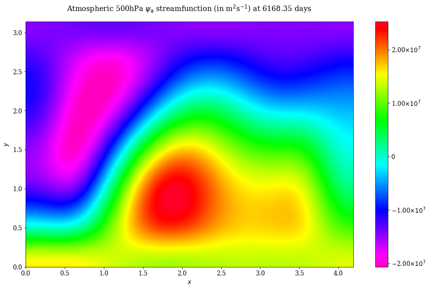
For instance, we can define a MiddleAtmosphericStreamfunctionDiagnostic diagnostic that returns the
500hPa streamfunction field:
psi_a = MiddleAtmosphericStreamfunctionDiagnostic(model_parameters)
and feed it with a model outputs time and trajectory previously computed
(like in the previous section):
psi_a.set_data(time, trajectory)
It is then possible to plot the corresponding fields with the plot() method:
psi_a.plot(50)
or to easily create animation widget and movie of the diagnostic with
respectively the animate() and movie() methods:
psi_a.movie(figsize=(13,8), anim_kwargs={'interval': 100, 'frames':100})
All the diagnostics classes should in principle have these 3 methods
(plot, animate and movie). Note that the movies can also be
saved in mpeg 4 format.
One can also define multiple diagnostics and couple them toghether with
a MultiDiagnostic object. For instance, here we couple the previous psi_a
diagnostic with a dynamical scatter plot:
variable_nondim = VariablesDiagnostic([2, 1, 0], model_parameters, False)
m = MultiDiagnostic(1,2)
m.add_diagnostic(variable_nondim, diagnostic_kwargs={'show_time':True, 'style':'2Dscatter'}, plot_kwargs={'ms': 0.2})
m.add_diagnostic(psi_a, diagnostic_kwargs={'show_time':False})
m.set_data(time, trajectory)
As with the other diagnostics, the MultiDiagnostic object can plot
and create movies:
m.plot(50)
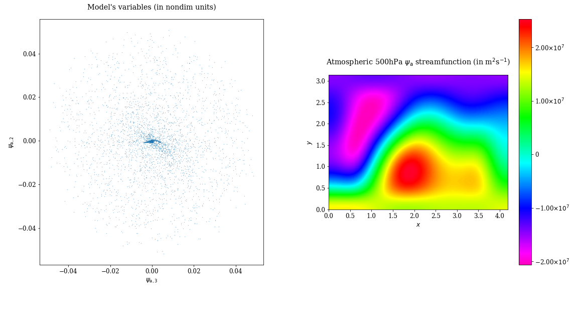
m.movie(figsize=(15,8), anim_kwargs={'interval': 100, 'frames':100})
Further examples using the diagnostics can be found in the sections Recovering the result of Reinhold and Pierrehumbert (1982),
Recovering the result of De Cruz, Demaeyer and Vannitsem (2016) and Manual setting of the basis.
Examples are also provided in the in the notebooks folder.
Moreover, the diagnostics classes methods are fully described in the section Diagnostics of the References.
Full list of currently available diagnostics
MiddleAtmosphericTemperatureAnomalyDiagnostic: Diagnostic giving the middle atmospheric temperature anomaly fields \(\delta T_{\rm a}\).
MiddleAtmosphericTemperatureDiagnostic: Diagnostic giving the middle atmospheric temperature fields \(T_{\rm a}\).
MiddleAtmosphericTemperatureMeridionalGradientDiagnostic: Diagnostic giving the meridional gradient of the middle atmospheric temperature fields \(\partial_y T_{\rm a}\).
OceanicLayerTemperatureAnomalyDiagnostic: Diagnostic giving the oceanic layer temperature anomaly fields \(\delta T_{\rm o}\).
OceanicLayerTemperatureDiagnostic: Diagnostic giving the oceanic layer temperature fields \(T_{\rm o}\).
GroundTemperatureAnomalyDiagnostic: Diagnostic giving the ground layer temperature anomaly fields \(\delta T_{\rm g}\).
GroundTemperatureDiagnostic: Diagnostic giving the ground layer temperature fields \(T_{\rm g}\).
LowerLayerAtmosphericStreamfunctionDiagnostic: Diagnostic giving the lower layer atmospheric streamfunction fields \(\psi^3_{\rm a}\).
UpperLayerAtmosphericStreamfunctionDiagnostic: Diagnostic giving the upper layer atmospheric streamfunction fields \(\psi^1_{\rm a}\).
MiddleAtmosphericStreamfunctionDiagnostic: Diagnostic giving the middle atmospheric streamfunction fields \(\psi_{\rm a}\).
OceanicLayerStreamfunctionDiagnostic: Diagnostic giving the oceanic layer streamfunction fields \(\psi_{\rm o}\).
VariablesDiagnostic: General class to get and show the scalar variables of the models.
GeopotentialHeightDifferenceDiagnostic: Class to compute and show the geopotential height difference between points of the model’s domain.
AtmosphericWindDiagnostic: General base class for atmospheric wind diagnostic.
LowerLayerAtmosphericVWindDiagnostic: Diagnostic giving the lower layer atmospheric V wind fields \(\partial_x \psi^3_{\rm a}\).
LowerLayerAtmosphericUWindDiagnostic: Diagnostic giving the lower layer atmospheric U wind fields \(- \partial_y \psi^3_{\rm a}\).
MiddleAtmosphericVWindDiagnostic: Diagnostic giving the middle atmospheric V wind fields \(\partial_x \psi_{\rm a}\).
MiddleAtmosphericUWindDiagnostic: Diagnostic giving the middle atmospheric U wind fields \(- \partial_y \psi_{\rm a}\).
UpperLayerAtmosphericVWindDiagnostic: Diagnostic giving the upper layer atmospheric V wind fields \(\partial_x \psi^1_{\rm a}\).
UpperLayerAtmosphericUWindDiagnostic: Diagnostic giving the upper layer atmospheric U wind fields \(- \partial_y \psi^1_{\rm a}\).
LowerLayerAtmosphericWindIntensityDiagnostic: Diagnostic giving the lower layer atmospheric horizontal wind intensity fields.
MiddleAtmosphericWindIntensityDiagnostic: Diagnostic giving the middle atmospheric horizontal wind intensity fields.
UpperLayerAtmosphericWindIntensityDiagnostic: Diagnostic giving the upper layer atmospheric horizontal wind intensity fields.
MiddleLayerVerticalVelocity: Diagnostic giving the middle atmospheric layer vertical wind intensity fields.
MiddleAtmosphericEddyHeatFluxDiagnostic: Diagnostic giving the middle atmospheric eddy heat flux field.
MiddleAtmosphericEddyHeatFluxProfileDiagnostic: Diagnostic giving the middle atmospheric eddy heat flux zonally averaged profile.
LowerLayerAtmosphericVorticityDiagnostic: Diagnostic giving the lower layer atmospheric vorticity fields \(\nabla^2 \psi^3_{\rm a}\).
MiddleAtmosphericVorticityDiagnostic: Diagnostic giving the middle atmospheric vorticity fields \(\nabla^2 \psi_{\rm a}\).
UpperLayerAtmosphericVorticityDiagnostic: Diagnostic giving the upper layer atmospheric vorticity fields \(\nabla^2 \psi^1_{\rm a}\).
LowerLayerAtmosphericPotentialVorticityDiagnostic: Diagnostic giving the lower layer atmospheric potential vorticity fields \(\nabla^2 \psi^3_{\rm a} + f_0 + \beta\, y + \frac{f_0^2}{\sigma_0\, \delta p^2} \theta_{\rm a}\).
UpperLayerAtmosphericPotentialVorticityDiagnostic: Diagnostic giving the upper layer atmospheric potential vorticity fields \(\nabla^2 \psi^1_{\rm a} + f_0 + \beta\, y - \frac{f_0^2}{\sigma_0\, \delta p^2} \theta_{\rm a}\).
More diagnostics will be implemented soon.
5.2 Toolbox
The toolbox regroups submodules to make specific analysis with the model and are available in the qgs.toolbox module.
For the references of these submodules, see Toolbox module.
Presently, the list of submodules available is the following:
lyapunov: A module to compute Lyapunov exponents and vectors.
More submodules will be implemented soon.
5.2.1 Lyapunov toolbox
This module allows you to integrate the model and simultaneously obtain the local Lyapunov vectors and exponents. The methods included are:
The Benettin algorithm to compute the Forward and Backward Lyapunov vectors [USER-BGGS80]. This method is implemented in the
LyapunovsEstimatorclass.The method of the intersection between the subspaces spanned by the Forward and Backward vectors to find the Covariant Lyapunov vectors [USER-ER85] (see also [USER-DPV21]). Suitable for long trajectories. This method is implemented in the
CovariantLyapunovsEstimatorclass.The Ginelli method [USER-GPT+07] to compute also the Covariant Lyapunov vectors. Suitable for a trajectory not too long (depends on the memory available). This method is also implemented in the
CovariantLyapunovsEstimatorclass.
See also [USER-KP12] for a description of these methods.
Some example notebooks on how to use this module are available in the notebooks/lyapunov folder.
6. Developers information
6.1 Running the test
The model core tensors can be tested by running pytest in the main folder:
pytest
This will run all the tests and return a report. The test cases are written using unittest. Additionally, test cases can be executed separately by running:
python -m unittest model_test/test_name.py
E.g., testing the MAOOAM inner products can be done by running:
python -m unittest model_test/test_inner_products.py
References
Giancarlo Benettin, Luigi Galgani, Antonio Giorgilli, and Jean-Marie Strelcyn. Lyapunov characteristic exponents for smooth dynamical systems and for hamiltonian systems; a method for computing all of them. part 1: theory. Meccanica, 15(1):9–20, 1980. URL: https://link.springer.com/article/10.1007/BF02128236.
L. De Cruz, J. Demaeyer, and S. Vannitsem. The Modular Arbitrary-Order Ocean-Atmosphere Model: MAOOAM v1.0. Geoscientific Model Development, 9(8):2793–2808, 2016. URL: https://www.geosci-model-dev.net/9/2793/2016/.
Jonathan Demaeyer, Stephen G Penny, and Stéphane Vannitsem. Identifying efficient ensemble perturbations for initializing subseasonal-to-seasonal prediction. arXiv preprint arXiv:2109.07979, 2021. URL: https://arxiv.org/abs/2109.07979.
J-P Eckmann and David Ruelle. Ergodic theory of chaos and strange attractors. The theory of chaotic attractors, pages 273–312, 1985. URL: https://link.springer.com/chapter/10.1007/978-0-387-21830-4_17.
Francesco Ginelli, Pietro Poggi, Alessio Turchi, Hugues Chaté, Roberto Livi, and Antonio Politi. Characterizing dynamics with covariant lyapunov vectors. Physical review letters, 99(13):130601, 2007. URL: https://journals.aps.org/prl/abstract/10.1103/PhysRevLett.99.130601.
Pavel V Kuptsov and Ulrich Parlitz. Theory and computation of covariant lyapunov vectors. Journal of nonlinear science, 22(5):727–762, 2012. URL: https://link.springer.com/article/10.1007/s00332-012-9126-5.
S. Pierini. Low-frequency variability, coherence resonance, and phase selection in a low-order model of the wind-driven ocean circulation. Journal of Physical Oceanography, 41(9):1585–1604, 2011. URL: https://journals.ametsoc.org/doi/full/10.1175/JPO-D-10-05018.1.
S Vannitsem and L De Cruz. A 24-variable low-order coupled ocean–atmosphere model: OA-QG-WS v2. Geoscientific Model Development, 7(2):649–662, 2014. URL: https://gmd.copernicus.org/articles/7/649/2014/.
S. Vannitsem, J. Demaeyer, L. De Cruz, and M. Ghil. Low-frequency variability and heat transport in a low-order nonlinear coupled ocean–atmosphere model. Physica D: Nonlinear Phenomena, 309:71–85, 2015. URL: https://www.sciencedirect.com/science/article/abs/pii/S0167278915001335.
Footnotes